How to import or export LaTeX equation into MS Word Equation or into MathType or with freewares?; special symbols; formula editors, plug-in; import/export with microsoft office (word, powerpoint)

Converters from or to LaTeX from or to Textprocessors or powepoint-like programs (MS office or other) - Overview

A formula editor is a name for a computer program that is used to typeset mathematical works or formulae in a web browser, stand alone, plug-in for microsoft office, or general plug-in (for example Mathtype
works with 400 applications and websites.
http://en.wikipedia.org/wiki/Formula_editor
Content for formula editors can be provided manually using a markup language, e.g. TeX or MathML, via a point-and-click GUI (mathtype), or as computer generated results from symbolic computations such as Mathematica.


Oldies: Microsoft Equation Editor 3.0 is a deprecated editor included in Microsoft Office products, based on limited version of MathType (US$57 academic).
Now: Microsoft Equation Editor  with MS office 2011
MAC: Equation Editor.app  v14.2.0 (august 2010) 4MB (Intel version)
also a limited version of MathType.
See below for how to use the full version of MathType which allows many import/export.


To illustrate these, let me restrict it to the Microsoft Word case:

• directly type or paste LaTeX code into Word 
• use a Word import filter 
• use a Word macro: load LaTeX file as plain text, then search for LaTeX markup and replace the markup by formatting, special characters and equations. 
• use an external converter:

1. LaTeX -> RTF, then use Word's own RTF import,
2. LaTeX -> HTML, then use Word's internet assistant or built-in html converter,
3. maybe other external format(s).

The converters being most complete and currently maintained / supported are:
TeX2Word - a shareware LaTeX import filter for MS Word
GrindEQ - a shareware LaTeX import filter for MS Word
latex2rtf - a free standalone LaTeX -> RTF converter for PC, Macintosh and Unix,
TeX4ht - a free LaTeX to html or XML converter for PC and Unix produces html which is good for loading into Word. TeX4ht relies on other software, it needs at least a full TeX system.

Directly type or paste LaTeX code into Word

All of these only allow typing or pasting LaTeX coded equations in Word, not LaTeX coded text elements.
"Aurora" can now convert a LaTeX coded equation (which must be placed on the Windows clipboard) to Word. The converter is still experimental and as such has a number of limitations, some of which will be addressed in future releases. The converter’s output will generally need some manual touching up to achieve the level of fidelity on a par with the original document.
The other functionality of Aurora, which was the only functionality of its predecessor "Ribbit", is letting you enter LaTeX equations in word processors such as MS Word or in Powerpoint. One can enter the equation in LaTeX markup, and the formatted equation is inserted as an object.
See homepage (external link) (Shareware)
Aurora needs a working LaTeX installation. If there is no, it will install a micro version of MiKTeX.

"LaTeX in Word": See homepage (external link) (Freeware, GPL).
It allows to enter LaTeX equations in word processors such as MS Word in LaTeX markup, and the formatted equation is inserted in the Wordprocessor as a png bitmap. It needs a server which performs the conversion. Server installation files are available from the download page (external link).

MathType (external link) allows typing and pasting equations in LaTeX markup and also direct conversion of an equation in LaTeX markup which is part of the Word document text.
OpenOffice allows typing equations in LaTeX-like markup.
Word 2007 allows typing equations in LaTeX-like markup (although not 100% compatible), see http://blogs.msdn.com/microsoft_office_word/archive/2006/10/04/Equations-in-Word-2007.aspx


Typing equations from the keyboard:

• Create and edit equations using only the keyboard and without leaving Word: MathType adds keyboard shortcuts to Word that allow you to insert a new equation, or edit an existing one, using just a keystroke.
• Type equations in TeX directly into Word: You can type TeX directly into Word. When you are done, type Alt+\ (Toggle TeX) to convert it to a MathType equation. Later, if you want to edit the equation's TeX code, just type Alt+\ again. The Toggle TeX command allows you to switch between TeX and MathType views of the equation.

MathType is a powerful interactive equation editor for Windows and Macintosh that lets you create mathematical notation for word processing, web pages, desktop publishing, presentations, elearning, and for TeX, LaTeX, and MathML documents.
MathType works with any wordprocessor, presentation program, page layout program, HTML-authoring tool and other types of software, to create perfectly formatted maths for class materials, research papers, web pages, slide presentations, journal articles and books.
Version 6.8 is loaded with features to help you do more, save time and create better-looking documents and web sites.
New features include:
MathType support for 64-bit Microsoft Office
Compatibility with 40 new apps (600+ and counting...)
Paste tables from spreadsheets, documents, web pages, etc. into MathType as a matrix (frequent user request)
MathPage support for Microsoft Word 2010 and 2007, converts documents into web pages, properly handling mathematical symbols.
Authoring for Accessibility: As part of our work in the accessibility community, we've made MathType useful for people with various disabilities, such as blindness, low vision, and learning disabilities.
Download Free Trial of MathType 6.8 for Windows. or MathType 6.7 for Mac.

Works with:

Microsoft Office, Apple iWork '09, Adobe InDesign, iBooks Author, Mathematica, Maple, GMail,OpenOffice, Blackboard, Moodle...



More Ways to Create Equations
Entering Maths by Hand: Entering equations as easily as you would write maths with paper and pencil! This feature uses the built-in handwriting recognition in Windows 7 or later.
Point-and-Click Editing with Automatic Formatting: Create equations quickly by choosing templates from MathType's palettes and typing into their empty slots. MathType applies mathematical spacing rules automatically as you type.
Keyboard Shortcuts: Save time using keyboard shortcuts. MathType has customisable keyboard shortcuts for virtually every symbol, template, and command.
Type TeX or LaTeX: If you already know the TeX typesetting language, you can enter equations directly into MathType or Microsoft Word documents. TeX editing can be mixed with point-and-click editing so you get the best of both worlds. You can even paste in equations from existing TeX documents.
http://www.dessci.com/en/products/mathtype/features.htm#mathml_import
Copy-and-Paste: If you created your equation in another application or found one on a website, why take the time to create it by hand again? Simply Copy-and-Paste it directly into MathType, and it is ready to edit or use in your work.
Save Expressions in the Toolbar: Drag frequently used equations and expressions to the MathType toolbar so they can be inserted later with just a click or a keystroke.
Supports Microsoft Office 2010 (both 32- and 64-bit), 2007, 2003, and XP (2002)
Microsoft Office 2007 & 2010 — MathType Ribbon Tab in Word and PowerPoint: MathType takes full advantage of Office's Ribbon User Interface making it easier than ever to do equation operations in documents and presentations. New equation numbering and browse features work with all Word equation types.
Microsoft Office 2003, XP (2002) — MathType Toolbar and Menu in Word and PowerPoint: MathType adds a toolbar and menu to Microsoft Word and PowerPoint, allowing quick access to its features and powerful commands to do equation numbering, produce great-looking maths web pages, presentations, and much more.
Find Symbols: MathType's Insert Symbol dialog allows you to explore the available symbols and insert them with a click or keystroke. 
More Control:
Colour: Use colour to highlight part of an equation and focus your audience's attention on just the portions you want. Show what changed in each step of a multi-step procedure and make those equations really come to life.
More Fonts: MathType has hundreds more symbols and templates than Equation Editor. Besides our exclusive Euclid™ maths fonts, you can also make use of the 1000s of maths symbols in fonts already on your computer, as well as other maths fonts you can download from the Internet.
System Requirements:
Windows: Microsoft Windows 7, Windows Vista, or Windows XP.
12 MB free hard disk space. MathType is not RAM-intensive so listing its requirements is not necessary.
Macintosh: Mac OS X 10.3.9 or newer. 20 MB free hard disk space.


If you are using OS X, one of my preferred solution is LaTeXiT, which creates a picture of the equation that you can drag into Word or elsewhere. A potential Windows analog that I have not tested is Laeqed.

Some solutions for MS powerpoint:

https://sites.google.com/site/tex4ppt/

TeXPPT is a lightweight add-in for Microsoft PowerPoint that lets you input LaTeX source code directly in your presentations.

Rendered LaTeX code becomes true PowerPoint shapes (i.e. vector graphics) which can be manipulated as such: you can resize, colorize, drop shadows and even animate them without loosing quality! Furthermore, TeXPPT does not have to be installed in order to view a PowerPoint presentation containing LaTeX objects.

TeXPPT requires a working installation of MiKTeX, Ghostscript and pstoedit.If you don't want to mess with the PATH environment variable, you should install the 32-bit version of Ghostscript otherwise pstoedit won't find it automatically. It works with PowerPoint 2007 or 2010. You might need to install the .NET Framework 4 manually. If the installer complains about security issues, the signing certificate is available here. Simply double click to install the certificate.

http://thd.pnpi.spb.ru/~gromov/mytexpoint.html

MyTeXPoint (absolutely Free)

Free simplified version of TeXPoint. Partly compatible with the original TeXPoint.

It has integrated screenshot tool to copy equations and pictures right from the screen.

Supports microsoft powerpoint (tested with version 2007 and 2005). Compatible with Microsoft Office 2010.

MyTexPoint est une version simplifiee et gratuite de TexPoint. Cette version est partiellement compatible avec TexPoint MyTexPoint donne la possibilite de creer des formules mathematiques en utilisant Latex, et de les inserer dans des presentations. MyTexPoint possede differents outils de Latex et est, pour l'instant, seulement compatible avec Microsoft Powerpoint. 

How to use MyTexPoint

1) Open you presentation.

2) When powerpoint is open run mytexpoint.

3) Click on the "new equation" button (the last one). A new equation will appear. You can edit its LaTeX code in the mytexpoint window.

4) To copy an equation or picture right from the screen use the first button.

5) To delete white background from an arbitrary picture in your power point presentation select it in the power point and doubleclick on the mytexpoint window.

Shortcuts:

Compile	Shift+Enter or Ctrl+Shift+L
New equation	Ctrl+N
Jump between equations	Ctrl+PgUp and Ctrl+PgDown
Move equations	Ctrl+arrows
Resize equations	Ctrl+Shift+arrows
Move equations a bit	Alt+arrows
Resize equations a bit	Alt+Shift+arrows

 Make sure that you have MiKTex and ghostscript installed

Vector picture formats (requeres pstoedit)

http://www.technion.ac.il/~zvikabh/software/iguanatex/

IguanaTex: a Free LaTeX Add-In for PowerPoint

IguanaTex is a PowerPoint plug-in which allows you to insert LaTeX equations into your PowerPoint presentation.

Select New Latex Equation from the Insert menu, and you will get a dialog box where you can type your equation. Type any valid LaTeX code, and click on Create. IguanaTex will compile your code into LaTeX, create an image from it and insert it into PowerPoint.

Need to change something in the equation? Just double-click on the image, and the IguanaTex dialog will re-appear so you can edit the LaTeX code; or, select the image and choose Edit Latex Equation from the Insert menu.

You can also treat the equation as an ordinary PowerPoint image. For example, it can be animated, rotated, moved, and resized.

When you save the presentation, both the image and the LaTeX code are stored. This means that you can display your presentation on any computer, even computers on which IguanaTex is not installed (no more missing fonts!). Of course, equations can only be edited if you install IguanaTex.

System Requirements

Windows 2000 or later, also support 64-bit versions of Windows.

PowerPoint: IguanaTex has been tested with PowerPoint 2000, 2003, 2007, and 2010.

LaTeX (can be downloaded from here: http://miktex.org/)

"not free" solutions:

http://texpoint.necula.org/buy.html

30 US$

Full integration with Powerpoint and Word, in several languages

Authors:

George Necula (University of California, Berkeley)

Andreas Glatz (Argonne National Laboratory).

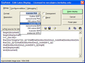
Using EMF Displays (Windows only)

Starting in version 2.0 of TexPoint you can create displays that are not bitmaps but outline graphics format (like PDF or Postscript). The actual graphics format is called EMF (Extended Metafile). To create such a display you must make sure to have installed the "Outline displays" feature of TexPoint (available and installed unless prohibited by you, starting with version 2.0). If you have this feature installed then you will see the EMF option in the "Bitmap format" combo box when you create or edit a display

TexPoint uses the PSTOEDIT program to translate the Postscript files generated by Latex into EMF. The program pstoedit.exe is installed in the TexPoint directory.  (To see the generated EMF file you can check the "Debugging/Keep Files" box and then look into the directory that contains the presentation. You will see that these files are much smaller than the bitmap files for the same display.)

The way EMF files work is that instead of containing a bitmap rendering of the characters that make up your display they contain references to characters in True Type (.ttf) versions of the Latex fonts. The catch is that for the displays to show correctly those fonts must be installed in your system. Make sure you read how TexPoint deals with these fonts to ensure that your presentation is viewable on machines without TexPoint.

The pstoedit tool will fail to create the EMF file if it contains fonts that are not installed in the system. In that case you will see a dialog box listing the fonts that are missing. TexPoint gives you the option to let pstoedit to substitute missing fonts. Just click the "Allow font substitution" checkbox. Please let us know if this is failing for standard Tex fonts.

EMF displays are transparent by default and cannot be made otherwise.

Office 2000 users: PowerPoint 2000 "forgets" to close EMF files that it loads. This prevents TexPoint from deleting the EMF files and requires it to create new EMF files with new names. The new names are formed using the value you have in the Debugging pane (default is txp_fig) along with a random numeric suffix. It is Ok to delete these files manually after you exit PowerPoint. Their contents is already included in the presentation.

Mathtype

Equations Everywhere and Anywhere™
Work with math in over 400 applications and websites!

Install MathType 6.7 and MathType commands for Microsoft Office: the installer will automatically search  for Office installations. I tested in may 2012: it works with Microsoft office 2011 (Mac OSX 10.5.x--10.7).



Generate good-looking, accessible math web pages:
MathPage: MathType includes our MathPage™ technology that easily converts Microsoft Word documents into web pages, properly handling mathematical symbols as well as MathType and Equation Editor equations.
MathML or GIF: MathPage can generate equations as either GIF images or MathML. MathML will allow you to copy and paste math into many applications that understand MathML.
Exact Speech command: Overrides the automatically generated speech used by MathPlayer's math-to-speech or braille conversion for a selected expression or symbol. This is important in a number of situations, such as in an assessment situation where the normal speech text from screen readers or other accessible technology (AT) might give away the answer.
Math accessibility: MathML is the key to math accessibility, allowing equations in web pages to be spoken by screen readers that are used by the blind and others.

some screenshots of the files:

--------many import/export and many preferences:

the 5nd button: toggle between latex or rendering

---------
ex-ample: latex->toggle button->rendering 

---------------------------------------
http://superuser.com/questions/202806/how-to-import-latex-equation-into-ms-word-equation-or-into-mathtype


----------in french:
comment écrire un code algorithmique avec des équations dans des boites en utilisant word comme éditeur de text?


Je suis entrain d'écrire un article j'ai trouvée un problème avec latex, donc j'ai décidée d'utiliser word 2011. Le problème est que j'ai des codes algorithmiques que je vais l'introduire dans mon article, alors comment écrire un code algo en utilisant word comme éditeur de texte.

Spherical harmonics, meshes and some WebGL and JavaScript : toxiclibs.js, Processing.js, Three.js, ThreeNodes.js

1--------Spherical Harmonics Mesh Builder

http://www.chromeexperiments.com/detail/spherical-harmonics-mesh-builder/?f=

Spherical Harmonics Mesh Builder is an example of Paul Bourke's "spherical harmonics" function for creating organic meshes. This example shows the use of Toxiclibs.js for creating meshes inside Three.js

(Technology: JavaScript, WebGL, toxiclibs.js, three.js).

Spherical harmonics are the angular portion of a set of solutions to Laplace's equation. Spherical harmonics are important in many theoretical and practical applications, particularly in the computation of atomic orbital electron configurations, representation of gravitational fields, geoids, and the magnetic fields of planetary bodies and stars, and characterization of the cosmic microwave background radiation. In 3D computer graphics, spherical harmonics play a special role in a wide variety of topics including indirect lighting (ambient occlusion, global illumination, precomputed radiance transfer, etc.) and recognition of 3D shapes.

The 19th century development of Fourier series made possible the solution of a wide variety of physical problems in rectangular domains, such as the solution of the heat equation and wave equation. This could be achieved by expansion of functions in series of trigonometric functions. Whereas the trigonometric functions in a Fourier series represent the fundamental modes of vibration in a string, the spherical harmonics represent the fundamental modes of vibration of a sphere in much the same way.

is called a spherical harmonic function of degree ℓ and order m.

For a given value of ℓ, there are 2ℓ+1 independent solutions of this form, one for each integer m with −ℓ ≤ m ≤ ℓ. 

A quite good article http://en.wikipedia.org/wiki/Spherical_harmonics

and in french: http://fr.wikipedia.org/wiki/Harmonique_sph%C3%A9rique

http://mathworld.wolfram.com/SphericalHarmonic.html

http://demonstrations.wolfram.com/NodalDomainsOfSphericalHarmonics/

2------------http://haptic-data.com/

http://haptic-data.com/sketches/simplex_trails.html

http://haptic-data.com/toxiclibsjs/

Toxiclibs.js is an open-source computational design library ported to javascript by Kyle Phillips originally written by Karsten Schmidt for Java and Processing. Examples of the original library can be found at http://toxiclibs.org

Toxiclibs.js works great with Canvas, with SVG or any ordinary DOM element. with Processing.js, Three.js, or Raphael.js for SVG...

great example with additive waves

http://haptic-data.com/toxiclibsjs/examples/AdditiveWaves_pjs-webgl.html

3--------three.js

https://github.com/mrdoob/three.js

JavaScript 3D library

The aim of the project is to create a lightweight 3D library with a very low level of complexity — in other words, for dummies. The library provides ,

--ThreeNodes.js

http://idflood.github.com/ThreeNodes.js/public/index.html

Threenodes.js is an attempt to create a dataflow environment in javascript and html5. It's a way to see what is possible to do in the browser. I had a little list of interesting javascript libraries to try but never had the chance to play with them.

The project is still in an experimental state but you can already see a live demo there: http://idflood.github.com/ThreeNodes.js/

coffeescript, compass and haml
These are languages that compile to javascript, css and html. Their syntax are much shorter than their equivalent and they offer some great features. If you work a lot with js, css or html you should definitely check these.
http://jashkenas.github.com/coffee-script/
http://compass-style.org/
http://haml-lang.com/

Three.js
The project is using webgl to render the scene. Three.js was obviously the 3d engine of choice. It provide many features like shaders, geometries, postprocessing filters and so on. A great project :)
https://github.com/mrdoob/three.js/

node.js
This is a javascript server. It's used to automatically compile the source files and serve them. I could have used some simple bash script to compile the files but found it would be interesting to use this for this "node" based project.
http://nodejs.org/

Require.js
The application was quickly growing and I needed a way to make it more modular. It's still not used at his full potential in threenode.js but already help make the code cleaner. One nice feature is that it's possible to require text files, or in this case little html template files.
http://requirejs.org/

--------------

http://processingjs.org/

Processing.js is the sister project of the popular Processing visual programming language, designed for the web. Processing.js makes your data visualizations, digital art, interactive animations, educational graphs, video games, etc. work using web standards and without any plug-ins. You write code using the Processing language, include it in your web page, and Processing.js does the rest. It's not magic, but almost.

magnetic therapy/stimulation and hemoglobin-red blood cell-capillaries; the Magnetic permeability and the magnetic reluctivity and the magnetic susceptibility ; Latex and maxwell's equations; magnetism, magnet, electromagnet, Static and Stationary Magnetic Fields

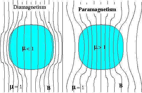
 In this figure µ (usually µr) is the "dimensionless" number µ/(µ0).
The term of "permeability" was coined in September, 1885 by Oliver Heaviside. 

Rem: 1)all equations are in png with latex in the alt (just right clic on the image to get the code).
2) all the figure contain its URL (auto-bibliography; or sometimes i put the URL below the figure).

This post is a short comment about µ which is the magnetic permeability (and also a compliation of wikipedia and others sites)
It is not easy to define µ and to understand this quantity.
en.Wikipedia : http://en.wikipedia.org/wiki/Magnetic_permeability
and in the case of vacuum: http://en.wikipedia.org/wiki/Vacuum_permeability
Try with other langages.wikipedia  (each x.wikipedia are different encyclopedia and  depand on wikipedians ;)

Permeability is the measure of the ability of a material to support the formation of a magnetic field within itself.

The reciprocal of magnetic permeability is magnetic reluctivity.

Graphical illustration of  the equation B=µH. Simplified comparison of permeabilities for: ferromagnets (μ_f), paramagnets(μ_p), free space(μ₀) and diamagnets (μ_d). This µf is not scaled (in fact it is near of the B-axis).

The auxiliary magnetic field H represents how a magnetic field B influences the organization of magnetic dipoles in a given medium, including dipole migration and magnetic dipole reorientation. Its relation to permeability is

where μ is a scalar if the medium is isotropic or a second rank tensor for an anisotropic medium.
In this post we will assume that µ is a scalar, B and H will be on the same axis (just a comment: in the case of some new special metamaterials we can get a negative µ).

In terms of relative permeability, the magnetic susceptibility is:

χ_m = μ_r − 1.

χ_m, a "dimensionless" quantity, is sometimes called volumetric or bulk susceptibility, to distinguish it from χ_p (magnetic mass or specific susceptibility) and χ_M (molar or molar mass susceptibility).


The magnetization could be modeled as: M = χ_m H


Permeability a constant?
In general, permeability is not a constant (but near of a constant for most of materials), as it can vary with the position in the medium, the frequency of the field applied, humidity, temperature... Permeability as a function of electromagnetic frequency can take on real or complex values.

Table of 'microscopic' equations

Formulation in terms of total charge and current

Name	Differential form	Integral form
Gauss's law
Gauss's law for magnetism
Maxwell–Faraday equation (Faraday's law of induction)
Ampère's circuital law (with Maxwell's correction)

Ref: http://en.wikipedia.org/wiki/Maxwell%27s_equations

µ0 only appears in the Maxwell-Ampère's circuital law. If you use H (not B), it is hidden in H then this equation with B is better ;)

Good luck with units:
permeability is the inductance per unit length. In SI units, permeability is measured in henries per metre (H·m⁻¹ = J/(A²·m) = N A⁻²). H has dimensions current per unit length and is measured in units of amperes per metre (A m⁻¹). The product μH thus has dimensions inductance times current per unit area (H·A/m²). But inductance is magnetic flux per unit current, so the product has dimensions magnetic flux per unit area. This is just the magnetic field B, which is measured in webers (volt-seconds) per square-metre (V·s/m²), or teslas (T).

B the magnetic induction
the Laplace force (a macroscopic force on the wire, when a wire carrying an electrical current is placed in a magnetic field):


tesla=Newton/(A.m)=Newton/(C.(m/s)).
or F=qE then Volt=Newton/(C)
then tesla=Volt/(m/s)

Idl (or J.dV with J Ampere/m2 and dV m3) plays the same role of the electric charge "q" (or densityOfCharge*dV : (C/m3)*m3).

Because the tesla is so large in regards to everyday usage, common engineering practice is to report the strength of magnets in Gauss. 10 G = 1 mT (millitesla).

B perpendicular to F and to dl


H Magnetic field strength
A magnetic dipole is "a closed circulation of electric current" (Maxwell-Ampère's circuital law). The dipole moment has dimensions current times area, units ampere square-metre (A·m2), and magnitude equal to the current around the loop times the area of the loop. H is related to the magnetic dipole density. The H field at a distance from a dipole has magnitude proportional to the dipole moment divided by distance cubed which has dimensions current per unit length.Then without "dimensionless tricks" H is a quantity with many space effects : (A.m2)/m3. H has also a time effect (A= Coulomb/s).

Ampère is a very bad unit to understand something (but it is a very good units in regard to 1Newton and electrotechnics).

-----------------------------------------------
Now we will see the magnitude.
I separate this aspect clearly because it is the most important.
If we dont consider magnets and/or strong stationnary or transient electric currents, all the materials are, in apparence, not "interactive" with magnetic fields.





They are grouped by orders of magnitud:
   0.1 pT  - brain activity, human brain magnetic field:

      1 pT  - cardiac activity:
    20 µT  - strength of magnetic tape near tape head
    31 µT  - strength of Earth's magnetic field at 0° latitude (on the equator)
    58 µT  - strength of Earth's magnetic field at 50° latitude
    0.5 mT  - the suggested exposure limit for cardiac pacemakers
                    by American Conference of Governmental Industrial Hygienists (ACGIH)
    5 mT - the strength of a typical refrigerator magnet
    0.15 T - Sunspots. They are temporary phenomena on the photosphere of the Sun that appear visibly as dark spots compared to surrounding regions. They are caused by intense magnetic activity, which inhibits convection by an effect comparable to the eddy current brake, forming areas of reduced surface temperature.
    1.25 T - Magnetic field intensity at the surface of a neodymium magnet; strength of a modern neodymium-iron-boron (Nd2Fe14B) rare earth magnet. A coin-sized neodymium magnet can lift more than 9 kg, can pinch skin.
    1 T to 2.4 T - coil gap of a typical loudspeaker magnet
    1.5 T to 3 T - strength of medical magnetic resonance imaging systems in practice,
          experimentally up to 17 T
     5 T - The strongest fields encountered from permanent magnets are from Halbach spheres.
  45 T - strongest continuous magnetic field yet produced in a laboratory (Florida State University's National High Magnetic Field Laboratory USA, dec 1999; 34 tons). http://www.magnet.fsu.edu/mediacenter/news/pressreleases/1999december17.html

   91.4 T - strongest (pulsed) magnetic field yet obtained non-destructively in a laboratory (Forschungszentrum Dresden-Rossendorf. http://www.hzdr.de/db/Cms?pOid=33768&pNid=473

   2.8 kT - strongest (pulsed) magnetic field ever obtained (with explosives) in a laboratory (VNIIEF in Sarov, Russia, 1998). DOI: http://dx.doi.org/10.1109/PPC.1999.823621



Ref: http://en.wikipedia.org/wiki/Orders_of_magnitude_%28magnetic_field%29

Magnetic levitation

   16 T - strength used to levitate a frog

              http://www.newscientist.com/article/mg15420771.600-frog-defies-gravity.html
The levitation trick works because giant magnetic fields slightly distort the orbits of electrons in the frog's atoms. The resulting electric current generates a magnetic field in the opposite direction to that of the magnet. A field of 16 teslas created an attractive force strong enough to make the frog float until it made its escape.
The team has also levitated plants, grasshoppers and fish. "If you have a magnet that is big enough, you could levitate a human," says Peter Main, one of the researchers.
He adds that the frog did not seem to suffer any ill effects: "It went back to its fellow frogs looking perfectly happy." 
A live frog levitates inside a 32 mm diameter vertical bore of a Bitter solenoid in a magnetic field of about 16 teslas at the High Field Magnet Laboratory of the Radboud University in Nijmegen the Netherlands:

http://www.youtube.com/watch?v=rotTjRY5lRw

Water possesses diamagnetic properties likewise, although less vivid, which makes the levitation of living beings, containing a large quantity of water, possible. So far the Henri Heim frog levitation experiment within the electromagnetic pair (1997) and the Jung Ming Lu mouse levitation experiment within the electric magnet (2009) have been a success (despite the former assumption of mammals being unable to levitate due to the differing ration of the liquid to the general body mass). 

 http://en.wikipedia.org/wiki/Andre_Geim

"The Frog That Learned to Fly". Radboud University Nijmegen.  For Geim's account of diamagnetic levitation. "Everyone's MagnetismPDF (688 KB). Physics Today. September 1998. pp. 36–39. For the experiment with Berry, see Berry, M. V.; Geim, Andre. (1997). "Of flying frogs and levitrons" PDF (228 KB). European Journal of Physics 18: 307–313.

http://en.wikipedia.org/wiki/Magnetic_levitation
Earnshaw's theorem proves that using only static ferromagnetism it is impossible to stably levitate against gravity, but servomechanisms, the use of diamagnetic materials, superconduction, or systems involving eddy currents permit this to occur.
All materials have diamagnetic properties, but the effect is very weak, and is usually overcome by the object's paramagnetic or ferromagnetic properties, which act in the opposite manner. Any material in which the diamagnetic component is strongest will be repelled by a magnet.
Earnshaw's theorem does not apply to diamagnets. These behave in the opposite manner to normal magnets owing to their relative permeability of μr < 1 (i.e. negative magnetic susceptibility).

Diamagnetic levitation can be used to levitate very light pieces of pyrolytic graphite or bismuth above a moderately strong permanent magnet. As water is predominantly diamagnetic, this technique has been used to levitate water droplets and even live animals, such as a grasshopper, frog and a mouse. However, the magnetic fields required for this are very high, typically in the range of 16 teslas, and therefore create significant problems if ferromagnetic materials are nearby.
The minimum criterion for diamagnetic levitation is

 where:

• ρ is the density of the material
• g is the local gravitational acceleration (−9.8 m/s² on Earth)
• is the rate of change of the magnetic field along the vertical axis.

Assuming ideal conditions along the z-direction of solenoid magnet:

• Water levitates at
• Graphite levitates at

Induced currents

These schemes work due to repulsion due to Lenz's law. When a conductor is presented with a time-varying magnetic field electrical currents in the conductor are set up which create a magnetic field that causes a repulsive effect.

Relative motion between conductors and magnets

If one moves a base made of a very good electrical conductor such as copper, aluminium or silver close to a magnet, an (eddy) current will be induced in the conductor that will oppose the changes in the field and create an opposite field that will repel the magnet (Lenz's law). At a sufficiently high rate of movement, a suspended magnet will levitate on the metal, or vice versa with suspended metal. Litz wire made of wire thinner than the skin depth for the frequencies seen by the metal works much more efficiently than solid conductors.
An especially technologically-interesting case of this comes when one uses a Halbach array instead of a single pole permanent magnet, as this almost doubles the field strength, which in turn almost doubles the strength of the eddy currents. The net effect is to more than triple the lift force. Using two opposed Halbach arrays increases the field even further.
Halbach arrays are also well-suited to magnetic levitation and stabilisation of gyroscopes and electric motor and generator spindles.

Oscillating electromagnetic fields

A conductor can be levitated above an electromagnet (or vice versa) with an alternating current flowing through it. This causes any regular conductor to behave like a diamagnet, due to the eddy currents generated in the conductor. Since the eddy currents create their own fields which oppose the magnetic field, the conductive object is repelled from the electromagnet, and most of the field lines of the magnetic field will no longer penetrate the conductive object.
This effect requires non-ferromagnetic but highly conductive materials like aluminium or copper, as the ferromagnetic ones are also strongly attracted to the electromagnet (although at high frequencies the field can still be expelled) and tend to have a higher resistivity giving lower eddy currents. Again, litz wire gives the best results.
The effect can be used for stunts such as levitating a telephone book by concealing an aluminium plate within it.
At high frequencies (a few tens of kilohertz or so) and kilowatt powers small quantities of metals can be levitated and melted using levitation melting without the risk of the metal being contaminated by the crucible.
-----

Just some comments about magnetic therapy [http://en.wikipedia.org/wiki/Magnet_therapy]:
Magnets produce energy in the form of magnetic fields. Two main types of magnets exist: static or permanent magnets, in which the magnetic field is generated by the spin of electrons within the material itself, and electromagnets, in which a magnetic field is generated when an electric current is applied. Most magnets that are marketed to consumers for health purposes are static magnets of various strengths, typically between 30 and 300 mT. Magnets have been incorporated into arm and leg wraps, mattress pads, necklaces, shoe inserts and bracelets.

The worldwide magnet therapy industry
The worldwide magnet therapy industry totals sales of over a billion dollars per year [http://news.bbc.co.uk/2/hi/health/4582282.stm], including $300 million dollars per year in the United States alone [http://www.csicop.org/si/show/magnet_therapy_a_billion-dollar_boondoggle/].

The ideas of "air du temps":
Even in the magnetic fields used in clinical magnetic resonance imaging, which are many times stronger of 300mT magnet ((i) 0.2 to 9.4 teslas static B and (ii) MegaHertz B), "none" of the claimed effects are observed [http://www.radiologyinfo.org/en/safety/index.cfm?pg=sfty_mr].

The TMS and rTMS is based on transient pulses of 1Teslas/(10-50microseconds) with 5000-8000Ampères/(10-50microseconds) in a coil. In this case some effects are clearly measured on the skin and "sometimes" on the surface of the cortex (e.g. motor cortex). The main effects seem to come from induced electric fields (the Maxwell–Faraday equation expresses that a time variation of B create an electric field: it is the induction).
http://en.wikipedia.org/wiki/Transcranial_magnetic_stimulation

There are many applications of induction (with high levels of B and E) and we need the transduction of eddy currents (courants de Foucault) and of Ohmic losses in special metals ("for induction") to increase the temperature...

There are a lot of controversies about magnet therapy:

Ref:  CMAJ September 25, 2007 vol. 177 no. 7 doi: 10.1503/cmaj.061344 

http://www.cmaj.ca/content/177/7/736.full

Hemoglobin, red blood cell and capillaries
Although hemoglobin, the blood protein that carries oxygen, is weakly  diamagnetic in the oxygenated
and weakly paramagnetic in the deoxygenated state (diamagnetic -> is repulsed by magnetic fields), the magnets used in magnetic therapy seems to be be many orders of magnitude too weak to have any measurable in vivo effect on blood flow.
At 500-600mT (static field), an effect on red blood cells microcirculation (a 40% decrease of RBC velocity  at 600mT @1.5mm in the tissue) was measured: http://www.ncbi.nlm.nih.gov/pubmed/17952798

[Brix, G. et al. Static magnetic fields affect capillary flow of red blood cells in striated skin muscle. Microcirculation 15, 15-26 (2008)]

It has been demonstrated that both normal [10, 11, 14, 35] and sickled [21] human erythrocytes are
aligned by SMF(statif magnetic fields) in cell suspensions. A highly significant orientation was also reported for sickled erythrocytes flowing through a 0.38T field in an in vitro flow apparatus [4]. In a series of experiments [10, 11, 35], Higashi and coworkers found that normal intact RBCs orient with their disk planes parallel to the magnetic field direction. Alignment was detectable at a flux density of 1T and almost 100% of the cells were oriented when exposed to 4T. Since orientation was not influenced by the spin state of hemoglobin (which is diamagnetic in the oxygenated
and paramagnetic in the deoxygenated state), it has been concluded that normal RBCs are oriented primarily due to the anisotropic diamagnetism of cell membrane components. On the other hand, estimations performed for normal RBCs by Schenck [25] indicate that the anisotropic diamagnetic susceptibility of single RBCs is probably too small to orient RBCs flowing in large vessels. These estimations, however, did not take into account that RBCs move in an oriented and deformed state through capillaries, which may change their anisotropic susceptibility (...)
In the case of dynamic RBC clustering, the SMF-induced torque, which increases with the number of anisotropic RBCs coupled, can be much larger than for single RBCs [25]. To obtain a deeper understanding of the observed effect of SMFs on microvascular blood flow, the existing computer models describing dynamic clustering of RBCs in capillaries should be extended to include the physical interaction of the different blood components with an external SMF.
As a first step in this direction, Haik et al. developed a simplified mathematical model, which couples orientation effects of RBCs with the shear stress by introducing a magnetically induced viscosity of blood that adds to the kinetic viscosity. In agreement with their theoretical considerations, the authors experimentally observed an increased viscosity of human blood flowing in a thin plastic tube when exposed to magnetic flux densities between 3 and 10 T as compared to measurements performed in the absence of a SMF [9; Haik Y, Pai V, Chen CJ. (2001). Apparent viscosity of human blood in a high static magnetic field. J Magn Magn Mater 225:180–186.]
Further work will be required to identify potential synergistic or alternative mechanisms by which SMFs are able to affect capillary RBC flow. For example, alterations of the endothelial glycocalyx or of the surface properties of RBCs may play an important role. It is widely recognized that the glycocalyx, a translucent layer with fixed negative charges, has manifold physiological functions. Crucial among these is its role as a hydrodynamic exclusion layer preventing the interaction of proteins in the RBCs and endothelial cell membranes; in modulating leukocyte attachment and rolling; and as a transducer of mechanical forces to the intracellular cytoskeleton in the initiation of intracellular signaling [31] (see also [16,29]). (...)
Muscle capillaries are mainly oriented in parallel and intersected perpendicularly by the magnetic field.(...)
Patients undergoing MR procedures at higher magnetic field strengths occasionally report on mild nausea and headache, which may possibly be related to an altered blood flow pattern [14; Kuchel PW, Coy A, Stilbs P. (1997). NMR “diffusion- diffraction’’ of water revealing alignment of erythrocytes in a magnetic field and their dimensions and membrane transport characteristics. Magn Reson Med 37:637–643].

---[Haik,2001; Apparent viscosity of human blood in a high static magnetic field;   http://dx.doi.org/10.1016/S0304-8853(00)01249-X]
Studying the effect of magnetic field on the blood is of interest to many researchers. Pauling and Coryell [1; 1936] were first to report the diamagnetic susceptibility of oxyhemoglobin and the paramagnetic susceptibility of deoxyhemoglobin. The value for the effective magnetic moments of the Fe²⁺ complex in hemoglobin of red blood cells is derived from their measurements. Higashi et al. [2] studied the orientation of normal erythrocytes in a strong static magnetic field with a maximum field strength of 8 T. The erythrocytes were found to orient with their disc plane parallel to the magnetic field direction. Yamagishi [3] reported a similar behavior of red blood cells at 4 T. Further, Yamagishi [3] found that platelets orient with the applied magnetic field at 3 T. We and others [3] have observed that fibrinogen, one of the plasma proteins, is polymerized and aligns with the applied field already at 4 T. Shalygin and coworkers [4] studied the behavior of erythrocytes in a high-gradient magnetic field. They reported that the susceptibility of the diamagnetic erythrocytes (oxygenated blood in artery) was found to be −(0.13–0.65)×10⁻⁸ cgs emu/cm³ Oe. For the paramagnetic (deoxygenated blood in vein) it was (13–33)×10⁻⁸ cgs emu/cm³ Oe. Similar results were reported by Haik and coworkers [5]. Motta et al. [6] reported orientation of the human hemoglobin when subjected to high magnetic field. Nakano et al. [7] reported that the torque needed to rotate an erythrocyte was very small when the magnetic field was rotating almost parallel to the heme planes in the unit cell, while it was very large when the magnetic field was oriented perpendicular to the heme planes. This demonstrates that the orientation of blood cells when subjected to a magnetic field is due to the magnetic torque. In this orientation, blood cells and the surrounding plasma fluid will interact and, combined with the magnetic force, increase the apparent viscosity of the blood.

--- [Cano,2006;Computer simulation of magnetic properties of human blood; Chemical Physics Letters 432 (2006) 548–552]
Shalygin et al. [6] studied the behaviour of erythrocytes under strong magnetic field gradients. These authors reported a susceptibility for diamagnetic erythrocytes of -(0.13–0.65)x10-8 cgs emu/cm3 Oe and (13–33)x10-8 cgs emu/cm3 Oe for paramagnetic erythrocytes.
From the point of view of the modelling of biological systems it is important to determine which are the basic molecular features that are necessary for a proper modelling. Over the years, primitive models have been very useful in the modelling of complex fluids by computer simulations [9]. In this Letter, we address the description of the magnetic susceptibility of blood using a primitive model comprised of a dipolar hard-spheres fluid (DHS) in the presence of a external field. We study two variations of this model, depending on the physical values used to reproduce the magnetic behaviour of human blood, either red blood cells or reduced hemoglobin molecules.

Following Ref. [8], we are going to consider the susceptibility per ml of substance. The magnetic susceptibility for whole blood, v, is given by
(7)

where χp and χd are the paramagnetic and diamagnetic susceptibility contributions, and mp and md are their fractions, respectively. The paramagnetic contribution arises from the deoxyhemoglobin, whereas the diamagnetic term is basically given by the susceptibility of water molecules, since 60% of blood solution is water [8]. Then, vd ~ 0.6 and χd = 0.6 χwater = -5.4x10-6. The susceptibility of whole human blood is χ = 3.5x10-6 [12]. Using these results in Eq. (7), an estimated value for χp is obtained,
χp =  2:2x10-5  (8)
This value agrees with reported data of χp, that has been determined within the range
-6.07x10-6 ≤ χp ≤ 2.2x10-5 [8,12–17]. Since
χp =nRC χRC  (9)
where nRC is the number of red cells contained within 1 ml of blood, nRC = 5x10^9 [18], and χRC is the magnetic susceptibility of a red blood cell, the magnetic susceptibility of a red blood cell is obtained using Eqs. (8) and (9),
χRC ~ 5x10-15
According to Eq. (5), the magnetization M of a RBC due to the effect of an external magnetic field H is given by
M =χRC H 
Assuming that the magnetization M is basically given by the dipolar moment of the cell, µRC
M = µRC/VRC
where VRC is the volume occupied by a RBC,
VRC = 9.0 x10-11 ml [18], then Eqs. (10)–(12) enable us to have a estimated value of µRC

---------

The relation between life and bio-magnet exists:
Science 23 December 2011: Vol. 334 no. 6063 pp. 1720-1723; DOI: 10.1126/science.1212596
A Cultured Greigite-Producing Magnetotactic Bacterium in a Novel Group of Sulfate-Reducing Bacteria
http://www.sciencemag.org/content/334/6063/1720.abstract
a comment in french: http://www.rtflash.fr/bacterie-produisant-nano-aimants-greigite-enfin-cultivee-en-laboratoire/article


Ref:
http://www.phys.lsu.edu/~jarrell/COURSES/ELECTRODYNAMICS_HTML/course_EM.html
Download: the Latex Source , the full Postscript or PDF notes , Randy's Mathematica examples [1,2,3,4], just the figures, the homework assignment, or the solutions.

Ref: for latex and Equation numbering
http://en.wikibooks.org/wiki/LaTeX/Advanced_Mathematics

A post (only in french) for tex-latex or xetex and é à ï î ç...; un post en français pour les caractères avec accents

This post is in french because it's focused on the use of french special characters with tex-latex ou xetex.
------intro:
Les caractères accentués et liés (é, à, æ, Å, ø…) n'existent pas en langue anglaise. De fait, le standard informatique ASCII « de base » ne définit que 127 caractères non accentués, dits « caractères ASCII 7 bits ». La norme ASCII définit des caractères étendus, dits « caractères 8 bits », pour chaque pays, ce qui permet d'avoir les caractères éccentués et liés directement sur le clavier. Unicode augmente encore ces aspects. Mais hélas Tex et Latex sont apparus avant unicode... Tout document texte LaTeX peut donc être écrit en ASCII 7bits, ce qui garantit la plus forte interopérabilité.
On va donc limiter ce post à Tex-Latex.


XeTeX (http://fr.wikipedia.org/wiki/XeTeX) est un logiciel de mise en page dérivé de TeX qui utilise l'Unicode et les technologies modernes de polices de caractères telles que OpenType. Initialement développé pour Mac OS X, il est maintenant multiplate-forme. Les fichiers sources sont, par défaut, en utf-8. XeTeX fonctionne avec LaTeX et ConTeXt (macro packages). Sa partie LaTeX est xelatex. Il est utilisé avec le package fontspec, qui permet une interface configurable pour le choix des fonts et permet un choix très vaste de fonts.
XeTeX est incorporé dans les distributions TeX Live 2010, MacTeX 2010 et MiKTeX 2.8.
Unicode et la norme ISO/CEI 10646 attribuent à chaque caractère un nom officiel au sein d’un répertoire commun unifié entre toutes les langues et tous les usages. Dès que le répertoire commun est approuvé, les caractères sont groupés en blocs en fonction de leur usage et des écritures supportées, et reçoivent une identification numérique unique appelée point de code, identifiée généralement sous la forme U+xxxx (où xxxx est un nombre hexadécimal de 4 à 6 chiffres, entre U+0000 et U+10FFFF). La plage définie permet d'attribuer jusqu'à 1 114 112 points de code.

Il y a aussi MathML voir sur ce blog la catégorie "mathML".

 ------généralités LaTeX
Les commandes commencent par une contre-oblique \ suivie de 2 possibilités:

• un nom composé uniquement de lettres non diacritiés.
  Une espace (en typographie, le mot « espace » est féminin…), un chiffre ou tout autre caractère clôture le nom,
  ex : x\mapsto2  ;
• un seul caractère spécial (non-lettre), ex : \#

Remarque: depuis janvier 2003, les formules mathématiques sur Wikipédia peuvent être écrites avec latex: http://fr.wikipedia.org/wiki/Aide:Formules_TeX
où les formules s'écrivent entre $\dots$.

------les caractères spéciaux (ascii non 7bits)
Les caractères suivant sont utilisés par LaTeX pour la compilation (ils ont une signification particulière pour la mise en forme du texte) et ne peuvent donc figurer tels quels dans le texte :

$ & % # { } _ \ ^ ~

Il faut les remplacer par d'autres. Il suffit de faire figurer une barre de fraction inversée « \ » devant,

\$ \& \% \# \{ \}

sauf pour les 3  caractères suivant (heureusement,  ils sont assez rarement utilisés en tant que tels):

« \ »	qui s'écrit	\ textbackslash,
« ~ »	"	\ textasciitilde,
« ^ »	"	\ textasciicircum.

Si l'on reste toujours sous le même environnement (même type d'ordinateur, même système d'exploitation, même pays), alors on peut utiliser les caractères accentués du clavier, quitte à utiliser l'extension inputenc en mettant :

\usepackage[latin1]{inputenc}

dans l'en-tête du fichier.
ou par exemple  \usepackage[frenchb]{babel} 
ou \usepackage[french]{babel}
Les deux sont absolument identiques mais frenchb indique clairement que l'on veut utiliser le français avec babel d'où le b. L'extension babel facilite l'adaptation de la typographie du document à sa langue comme calc permet d'accomplir des calculs simples. La liste des extensions est interminable ; heureusement, tous les paquetages sont réunis au sein du Comprehensive TeX Archive Network (CTAN).

Mais dans le cas général, si le texte doit être lu dans un autre environnement ou par quelqu'un d'un autre pays, il faut utiliser la frappe suivante avec les "commandes".

Pour mettre un accent aigü, il suffit de faire précéder la lettre de « \' », « \` » pour un accent grave, « \^ » pour un accent circonflexe, et « \" » pour un tréma. De manière générale, on a « \ + accent + lettre ».
Exemple :

é

\'e

É

\'E

è

\`e

à

\`a

È

\`E

À

\`A

ê

\^e

â

\^a

î

\^\i

ô

\^o

û

\^u

Ê

\^E

Â

\^A

Î

\^I

Ô

\^O

Û

\^U

ë

\"e

ï

\"\i

ü

\"u

Ë

\"E

Ï

\"I

Ü

\"U

NB : pour le « i » accentué, la barre de fraction entre l'accent et le i sert à enlever le point ; il est important de laisser un espace après le i, car certaines instruction commencent elles aussi par \i, comme \it (texte en italique) par exemple (cet espace sera ignoré lors de la compilation). Exemple :

ab\^\i me

pour écrire « abîme » Ajoutons la cédille, le « e dans l'a/o » et le symbole angström (unité de mesure des distances atomiques en physique) :

ç	\c c
Ç	\c C
æ	\ae
Æ	\AE
œ	\oe
Œ	\OE
Å	\AA

NB : pour la cédille, il est important de laisser un espace après le \c, car certaines instructions commencent elles aussi par \c, comme \chapter (marque le début d'un chapitre) par exemple (cet espace sera ignoré lors de la compilation). Exemple :

fa\c cade

pour écrire « façade » Voici quelques signes de ponctuation particuliers :

• petit tiret - (signe moins) : « - » ;
• tiret moyen – (de la largeur d'un « N ») pour les intervalles de nombres : « -- » ;
• tiret long — (de la largeur d'un « M ») pour les incides (alternative aux parenthèses) : « --- » ;
• guillemets français « et » : « << » et « >> » (deux signes inférieur et deux signes supérieur).

On peut aussi représenter les accent et caractères espagnols (tilde, points d'interrogation et d'exclamation inversés), norvégiens… Pour connaître les codes à taper, il faut chercher...
Enfin, il existe des caractères spéciaux pour la mise en page :

• l'espace insécable « ~ », qui n'est pas coupée par un changement de ligne et en français précède notamment les « : ; ! ? » (ces signes sont également suivis d'une espace normale) et se trouve à l'intérieur des guillemets et des tirets d'incise (qui sont eux-même encadrés par des espaces normales) ;
  en typographie française, on écrit …~;, …~!, …~?, <<~…~>> et ---~…~--- ;
• l'espace forcée « {} » (accolade d'ouverture-accolade de fermeture) ou bien « \  » (barre de fraction inversée-espace), qui est sécable ;
• et l'espace fine « \, ».

Notes

• 1 - ASCII : american standard code for instruction interchange retour
• 2 - un caractère est une lettre, un chiffre, mais aussi un signe de ponctuation, une espace… retour

 Ref: http://deuns.chez.com/latex/carac.html