Sometimes I have to put text on a path
Showing posts with label mesh. Show all posts

Saturday, May 19, 2012

Molecular visualization Off-Line and On-Line : spiderGL, a JavaScript 3D Graphics library which relies on WebGL for realtime rendering

http://spidergl.org/index.php

code: http://spidergl.org/js/spidergl.js
http://sourceforge.net/projects/spidergl/

GALLERY:
http://spidergl.org/code.php

1/ Web application, a shader authoring tool:

http://spidergl.org/meshade/index.html
code generation
(input just a mesh, file= .obj)

VERY GOOD.
Try it online or download the zipped archive (an HTTP server is needed):


2/ Visualization Methods for Molecular Studies on the Web Platform

http://vcg.isti.cnr.it/Publications/2010/CADZS10/
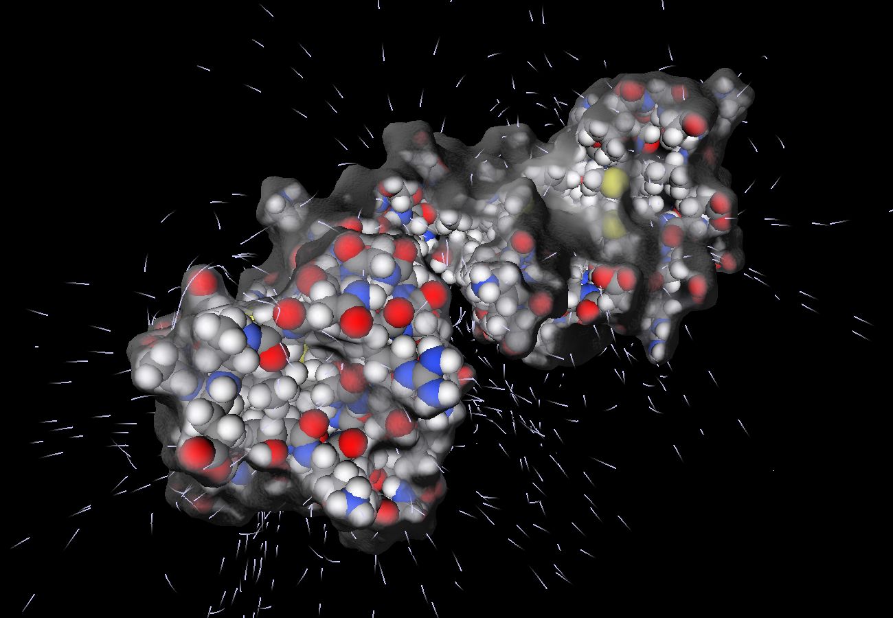


Standard representation of molecular surface properties using color ramps and field lines (leftmost), the same properties drawn using complex shading techniques (center) and the electrical interaction of two proteins (rightmost), rendered on a Web Page by using SpiderGL and WebGL.


Molecular visualization Off-Line and On-Line


The solution of the 3D structure of myoglobin in 1958 by Kendrew [Kendrew et al. 1958] marked the beginning of the new era of protein structural biology. Since then, a large number of protein structures have been solved and today the Protein Data Bank counts over 60.000 entries [Berman et al. 2003]. With the availability of all these data and the advance of computer graphics technologies, many research groups have developed tools for the manipulation and visualization of 3D structures such as VMD [Humphreyet al. 1996], SPDBViewer [Guex and Peitsch 1997], Chimera [Pettersen et al. 2004] and PyMOL [Delano 2002]. Beside working on the atomic structure, most programs can nowadays also calculate surface features such as electrostatic potential (using, for example, tools like APBS [Baker et al. 2001] or DelPhi [Rocchia et al. 2002]) and hydropathy [Kyte and Doolittle 1982].

In addition to the many standalone visualization tools, there are also web viewers especially designed for molecular structures, such as Jmol [jmo 2002] and MDL Chime, which represent a simple way
to visualize molecules directly on browser. MDL Chime, used by the Protein Explorer website was gradually phased out in favor of Jmol, which is nowadays the most used plugin for molecular visualization, used by websites such as Proteopedia and RCSB PDB Protein Data Bank.
Following the advance of techniques for the generation of CG movies, in the last few years many different groups focused on the creation of animated movies depicting biological molecules and
cellular processes. The movies range from the simple representations of the mechanical functioning of a single protein, to complex events involving many subjects. These works are important scientific efforts and add to their educational value the bonus of rising interest in the general public to approach biology. Some of these examples are collected on websites [McGill 2010; SCIVIS 2005].

3D Content on Web


The Virtual Markup Modeling Language (VRML) [Raggett 1994] (then replaced by X3D [Don Brutzmann 2007]) was proposed as a text based format for specifying 3D scenes in terms of geometry and material properties and for the definition of basic user interaction. The format itself was a standard, but the rendering in the web browser was relaying on specific plugins. The Java Applets are probably the most used method to add dynamic content, not necessarily 3D, in the web browsers. The
philosophy of Java applets is that the URL to the applet and its data are put in the HTML page and then executed by the Java Virtual Machine, a third part component. The implementation of JVM
on all the operating systems made Java applets ubiquitous and the introduction of binding to OpenGL such as JOGL [JOG ] added control on the 3D graphics hardware. A similar idea lies behind the
ActiveX [Microsoft Corporation 1996] technology, developed by Microsoft from 1996. Unlike Java Applets, ActiveX controls are not bytecode but dynamic linked Windows libraries which share
the same memory space as the calling process (i.e. the browser), and so much faster to execute. These technologies enable the incorporation of 3D graphics in a web page but they all do it by handling
a special element of the page itself with a third party component.


WebGL [Group 2009b] is an API specification produced by the Khronos group [Group 2009a] and, as the name suggests, defines the JavaScript analogous of the OpenGL API for C++. WebGL
closely matches OpenGLjES 2.0 and, extremely important, uses GLSL as the language for shader programs, which means that the shader core of existent applications can be reused for their
JavaScript/WebGL version. Since WebGL is a specification, it is up to the web browsers developer to implement it. At the time of this writing, WebGL is supported in the nightly build versions of the most used web browsers (Firefox, Chrome, Safari), and a number of JavaScript libraries are being developed to provide higher level functionalities to create 3D graphics applications. For example WebGLU [DeLillo 2009], which is the WebGL correspondent of GLU [OpenGL ARB ], provides wrappings for placing the camera in the scene or for creating simple geometric primitives, other libraries such as GLGE [Brunt 2010] or SceneJS [Kay 2009] uses WebGL for implementing a scene graph based rendering and animation engines.

Implementation spiderGL


Looking at a webpage with dynamic SpiderGL content, it is possible to see that all of the page logic is defined in the scripting part of the HEAD section, while on the BODY section there is just the page
structure and the interface elements that will be used for user interaction (like buttons, text areas and other controls). Among these elements, the most important is an html canvas object, that is the place where the WebGL layer does the on-screen rendering. ("< " are transformed : "[")

[canvas id="SGL_CANVAS" style="border: 1px solid gray"  width="900" height="600"][/canvas]


This canvas is registered as the output area at the end of the scripting; a specific function connects the various events of the canvas to a script object.


v a r  glMolViewer = new SpiderGLMolViewer ( ) ;
sglRegisterCanvas("SGL_CANVAS" , glMolViewer , 3 0 . 0 ) ;


The glMolViewer object is the main actor for the scene setup and rendering of our molecular visualization. The structure of this object employs the event handling subsystem provided by SpiderGL, which is inspired from the one used by the GLUT library [Kilgard ]. Each event coming from the canvas triggers a specific function with a given name and parameters; SpiderGL exploits the JavaScript language feature to give the possibility to dynamically add or remove listeners and redirect events. In this simple example, the only listener is the main object itself. (...)

This development process is straightforward for someone with an experience in graphical programming, while may prove to be difficult for users with a different background, like biology, physics or chemistry. This kind of setup is for sure more difficult to master with respect to setup of other existing platforms, like Jmol which, true to their nature, provide much simpler (but restrictive) access to their scene graph, with specific functions to import data and a series of predefined rendering modes. However, the gain in terms of flexibility and expressive power vastly compensate the initial steeper learning curve. Moreover, the learning of this technology is made easier by the possibility of initially use the higher level structures and functions implemented by SpiderGL to easily setup a basic visualization scheme and then start playing with lower level functions to obtain more complex effects. It is also important to note that most of the available JavaScript utility/UI libraries on the net may be used in conjunction with SpiderGL, adding more ready-made components to assemble a powerful, interactive, webpage.


3/ landscape refelction/refraction on a cup:

http://spidergl.org/example.php?id=12

This example uses how to use cube maps and spherical harmonics to render objects with a natural light effect. GOOD.

4/techno

SpiderGL: A JavaScript 3D Graphics Library for Next-Generation WWW


Monday, July 18, 2011

Is it possible to use a canvas to do 3d?; 3d web development with Google's O3D ; a canvas application which can read the contents of a 3D .OBJ file and display the results in real-time.


the new O3D Project Hosting site: http://code.google.com/p/o3d/

3d web development with Google's O3D: WebGL implementation of O3D

The old O3D plugin API is Deprecated:  
http://code.google.com/apis/o3d/docs/samplesdirectory.html

Originally built as a browser plug-in, this new implementation of O3D is a JavaScript library implemented on top of WebGL.


Introduction
The WebGL implementation of O3D is a JavaScript library built on top of WebGL. It implements a subset of the original O3D plug-in API, which includes all O3D interfaces that have an analogous interface in WebGL. For example, the render graph, transform graph, and texture classes are all implemented in the WebGL implementation of O3D. Animation, parameter operations, 2D canvas, and file I/O classes are not included. See Functional Groupings of O3D for details.

One major difference between the two implementations is that the WebGL implementation of O3D uses the GLSL shader required by WebGL. This release includes a Cg-to-GLSL converter script to aid in this conversion.


Here (http://code.google.com/p/o3d/) you can:
  • Download the WebGL implementation of O3D.
  • Read about how to convert your O3D plug-in application to the WebGL implementation of O3D.
  • Check out the samples.
  • Read about how to load COLLADA files into the WebGL implementation of O3D.
  • Browse the source code.
  • File bugs and submit patches.

--------------
O3D is a good development environment for 3d.
You will be surprised by how easy it was compared to OpenGL.
For example, entire 3d models could be loaded using a single command, while as with OpenGL you would have had to write your own low-level model loader.
Not to mention, Google made integration with Sketchup easy.

ex-ample:

http://src.chromium.org/viewvc/chrome/trunk/src/o3d/samples/o3d-webgl-samples


  • Hello Cube, v. 2
  • Spinning Cube, v. 2 (minimal changes)
  • Primitives, v. 2


http://code.google.com/p/o3d/wiki/SampleCodeWalkthrough

Converting and Loading COLLADA Models:
http://code.google.com/p/o3d/wiki/ColladaConverter

-------
"Is it possible to use a canvas to do 3d?"
3d and HTML5's Canvas element together...
The canvas element is becoming more widely adopted than O3D.  It could draw polygons.

The future of 3d web applications lies with WebGL : http://www.khronos.org/webgl/.
Using HTML5's canvas unlike WebGL: canvas will be able to run on any HTML5 enabled browser (software rendered) while as WebGL runs on computers with hardware acceleration.

Ex-ample:

3D OBJ Viewer – 3D, Applications - Canvas Demos:
http://www.canvasdemos.com/2010/05/05/3d-obj-viewer/
http://www.canvasdemos.com/userdemos/toxicgonzo/3dobjviewer.html
a canvas application which can read the contents of a 3D .OBJ file and display the results in real-time.
This particular demo takes Blender’s monkey model and rotates it. It also displays how many FPS in the upper left corner.

This program:
  1.  A 3d .OBJ object is stored as a string in the javascript file
  2. The .OBJ string is decoded to hold information about vertex position and which vertices form the polygons
  3.  Every polygon is assigned a random color
  4. Matrix multiplication happens: Convert object from model space -> camera space -> clip space -> screen space
  5.  Z-sort the polygons based on the polygon’s centroid
  6. Draw the polygons from back to front

Thursday, July 14, 2011

webGL skull (1162 faces) rendering.


http://www.chromeexperiments.com/detail/webgl-skull/?f=


Low poly normal mapped model exported from Blender, rendered in Three.js using Blinn-Phong shader with baked ambient occlusion texture, one directional and one point light.

Skull model by Daniel FR Gordillo:
http://www.blendswap.com/3D-models/misc-objects/craneo/
1162 faces, 924 KB total (including textures)
Technology: JavaScript, WebGL, Three.js, Blender

Friday, October 9, 2009

Mesh Generation & Grid Generation on the Web

http://www-users.informatik.rwth-aachen.de/~roberts/meshgeneration.html

Mesh Generation & Grid Generation on the Web


The aim of this document is to provide information on mesh and grid generation: people working in the field, research groups, books and conferences. It is maintained by Robert Schneiders.

Mesh generation is an interdisciplinary area, and people from different departments are working on it: Mathematicians, computer scientists, engineers from many disciplines. Despite the fact that surprisingly many people are active in the field, often there are few contacts between researchers. The aim of this page is to improve communication between research groups and to help people to get an overview of the field.

The page is organized as follows:

<!-- -->
    People and research groups: Info on meshing research at universities, companies, government labs etc. List of people: A directory of people working on mesh generation. Latest news: What's up in mesh generation. Software: A list of programs, both public domain and commercial. Conferences: Information on conferences, summerschools, short courses etc. Literature: Books, reviews, online sources and course materials. Open positions: Career opportunities for people with background in mesh generation. Information on related topics: Pages with information on CFD, scientific computing, computational geometry and other fields related to mesh generation.

<!-- --> Service for frequent readers: You can find all entries, sorted by time of insertion, here (there is also an archive page). <!-- Click here to see the latest updates (there is also an archive page). -->

Research on mesh generation is abundant, and I don't claim to give a complete overview. In order make this page a useful service for the mesh generation community, I need help from other people. So if you are interested in getting put on the list, or if you have any comments or hints on other sources of information on mesh generation in the net, please send me an email (robert.schneiders@arcor.de).

A valuable source of information is the Meshing Research Corner, a comprehensive database with literature on mesh generation. It is maintained by Steve Owen.

ParaView is an application framework as well as a turn-key application; Modeling software OpenFOAM and ParaView ; mesh processing: generation, manipulation, conversion

ParaView is an open source, multi-platform data analysis and visualization application. It has a client-server architecture to facilitate remote visualization of datasets

It is an application built on top of the Visualization Tool Kit (VTK) libraries.

The ParaView code base is designed in such a way that all of its components can be reused to quickly develop vertical applications. This flexibility allows ParaView developers to quickly develop applications.

Input/Output and File Format
  • Supports a variety of file formats including: VTK (new and legacy, all types including parallel, ascii and binary, can read and written).
  • Various polygonal file formats including STL and BYU (by default, read only, other VTK writers can be added by writing XML description).
  • Many other file formats are supported. See ParaView Readers and ParaView Writers for a full list.

CMake is a family of tools designed to build, test and package software. CMake is used to control the software compilation process using simple platform and compiler independent configuration files. CMake generates native makefiles and workspaces that can be used in the compiler environment of your choice. ParaView utilizes CMake for the software compilation process.

--------

ParaView is used as the visualization platform for the Modeling software OpenFOAM (Open Field Operation and Manipulation).It is primarily a C++ toolbox for the customisation and extension of numerical solvers for continuum mechanics problems, including computational fluid dynamics (CFD). It comes with a growing collection of pre-written solvers applicable to a wide range of problems.

First major general-purpose CFD package to use polyhedral cells. This functionality is a natural consequence of the hierarchical description of simulation objects.

OpenFOAM compares favourably with the capabilities of most leading general-purpose commercial closed-source CFD packages. It relies on the user's choice of third party pre- and post-processing utilities, and ships with:
  • a plugin (paraFoam) for visualisation of solution data and meshes in ParaView.
  • a wide range of mesh converters allowing import from a number of leading commercial packages
  • an automatic hexahedral mesher to mesh engineering configurations

OpenFOAM was conceived as a continuum mechanics platform but is ideal for building multi-physics simulations.

OpenCFD develop OpenFOAM in the Linux/UNIX operating system because: we believe it is the best platform for this kind of high end simulation code development and operation; Linux is efficient, robust, reliable and flexible and undergoes rapid development and improvement; Linux is open source, like OpenFOAM; Linux is very effective for parallel operation on Beowulf clusters.

OpenFOAM is open source software so people can freely compile it on any operating system they choose. Most OpenFOAM users are running Linux, so this site offers the download of binaries for selected Linux systems.

As the present time we are unaware of any binary distributions for Windows or MacOSX. However, ports to these operating systems have been the subject of debate on the OpenFOAM discussion site, which may provide the best source of information on the matter.

http://www.opencfd.co.uk/openfoam/

OpenFOAM uses finite volume numerics to solve systems of partial differential equations ascribed on any 3D unstructured mesh of polyhedral cells.

Mesh generation

OpenFOAM applications handle unstructured meshes of mixed polyhedra with any number of faces: hexahedra, tetrahedra, degenerate cells, basically anything.

Mesh generation is made simple by the fact that a cell is simply represented as a list of faces and a face as a list of vertices: this makes mesh handling very easy even for complex meshes with, say, embedded refinement or complex shapes near the boundary.

OpenFOAM is supplied with the following mesh generator tools that run in parallel.


Mesh generation tools


blockMesh A multi-block mesh generator
extrude2DMesh Takes 2D mesh (all faces 2 points only, no front and back faces) and creates a 3D mesh by extruding with specified thickness
extrudeMesh Extrude mesh from existing patch (by default outwards facing normals; optional flips faces) or from patch read from file
snappyHexMesh Automatic split hex mesher. Refines and snaps to surface


The main mesh generators cover two extremes: snappyHexMesh, that can mesh to complex CAD surfaces; blockMesh a simple file-driven block mesh generator.

Mesh manipulation

OpenFOAM is supplied with several utilties that perform mesh checking and manipulation. The full list of utilties is given below

Mesh manipulation


attachMesh Attach topologically detached mesh using prescribed mesh modifiers
autoPatch Divides external faces into patches based on (user supplied) feature angle
cellSet Selects a cell set through a dictionary
checkMesh Checks validity of a mesh
createBaffles Makes internal faces into boundary faces. Does not duplicate points, unlike mergeOrSplitBaffles
createPatch Utility to create patches out of selected boundary faces. Faces come either from existing patches or from a faceSet
deformedGeom Deforms a polyMesh using a displacement field U and a scaling factor supplied as an argument
faceSet Selects a face set through a dictionary
flattenMesh Flattens the front and back planes of a 2D cartesian mesh
insideCells Picks up cells with cell centre ’inside’ of surface. Requires surface to be closed and singly connected
mergeMeshes Merge two meshes
mergeOrSplitBaffles Detects faces that share points (baffles). Either merge them or duplicate the points
mirrorMesh Mirrors a mesh around a given plane
moveDynamicMesh Mesh motion and topological mesh changes utility
moveEngineMesh Solver for moving meshes for engine calculations.
moveMesh Solver for moving meshes
objToVTK Read obj line (not surface!) file and convert into vtk
pointSet Selects a point set through a dictionary
refineMesh Utility to refine cells in multiple directions
renumberMesh Renumbers the cell list in order to reduce the bandwidth, reading and renumbering all fields from all the time directories
rotateMesh Rotates the mesh and fields from the direcion n1   \special {t4ht= to the direction n2   \special {t4ht=
setSet Manipulate a cell/face/point set interactively
setsToZones Add pointZones/faceZones/cellZones to the mesh from similar named pointSets/faceSets/cellSets
splitMesh Splits mesh by making internal faces external. Uses attachDetach
splitMeshRegions Splits mesh into multiple regions
stitchMesh ’Stitches’ a mesh
subsetMesh Selects a section of mesh based on a cellSet
transformPoints Transforms the mesh points in the polyMesh directory according to the translate, rotate and scale options
zipUpMesh Reads in a mesh with hanging vertices and zips up the cells to guarantee that all polyhedral cells of valid shape are closed

Mesh motion

OpenFOAM adopts a novel approach to mesh motion by defining it in terms of the boundary motion which is extremely robust.

The solver need only define the the motion of the boundary and everything else will be done automatically. The open architecture of OpenFOAM solver codes allows quick and efficient implementation: mesh motion can be based on any solution variable, either local or integrated and by dynamically adjusted during the run.

Mesh motion is also transparently integrated with top-level models: the model writer does not see the additional complexity, which is conveniently packaged within the discretisation operators.

For examples of automated mesh motion in OpenFOAM, see Solutions

Mesh conversion

OpenFOAM accepts meshes generated by any of the major mesh generators and CAD systems. Listed below are converter utlities for the major commercial mesh generators. Note that it is also possible to import the meshes from most general purpose mesh generators since they will export in a format read by one of the converters.

Mesh converters


ansysToFoam Converts an ANSYS input mesh file, exported from I-DEAS, to OPENFOAM®format
cfx4ToFoam Converts a CFX 4 mesh to OPENFOAM®format
fluent3DMeshToFoam Converts a Fluent mesh to OPENFOAM®format
fluentMeshToFoam Converts a Fluent mesh to OPENFOAM®format including multiple region and region boundary handling
foamMeshToFluent Writes out the OPENFOAM®mesh in Fluent mesh format
foamToStarMesh Reads an OPENFOAM®mesh and writes a PROSTAR (v4) bnd/cel/vrt format
gambitToFoam Converts a GAMBIT mesh to OPENFOAM®format
gmshToFoam Reads .msh file as written by Gmsh
ideasUnvToFoam I-Deas unv format mesh conversion
kivaToFoam Converts a KIVA grid to OPENFOAM®format
mshToFoam Converts .msh file generated by the Adventure system
netgenNeutralToFoam Converts neutral file format as written by Netgen v4.4
plot3dToFoam Plot3d mesh (ascii/formatted format) converter
polyDualMesh Calculate the dual of a polyMesh. Adheres to all the feature and patch edges
sammToFoam Converts a STAR-CD SAMM mesh to OPENFOAM®format
star4ToFoam Converts a STAR-CD (v4) PROSTAR mesh into OPENFOAM®format
starToFoam Converts a STAR-CD PROSTAR mesh into OPENFOAM®format
tetgenToFoam Converts .ele and .node and .face files, written by tetgen
writeMeshObj For mesh debugging: writes mesh as three separate OBJ files which can be viewed with e.g. javaview

Thursday, October 8, 2009

mesh generation, literate programming, matlab; mathematica; persson

http://library.wolfram.com/infocenter/MathSource/5475/

This Mathematica notebook is an effort to transcribe the MATLAB code of a 2-D mesh generation algorithm as described explicitly in Persson and Strang's paper [1]. The goal is to make the algorithm executable in Mathematica so that its users can also experiment with the algorithm.

Since the algorithm was expressed very clearly from their original paper [1] including the MATLAB code, which is a perfect example of literate programming in MATLAB, it is pretty easy to translate the MATLAB code "literally" into Mathematica. Such translation is virtually always possible in either direction even without human interference. And such a Rosetta Stone kind of translation might be useful if one species of people coding in either MATLAB or Mathematica were to disappear, future generations would still be able to rediscover one programming language by reading its interpretation in the other one.

However, it is so tempting to present the literate programming capability of Mathematica by following its general principles; that is, (a) documentation mingles with code and both get pretty-printed; (b) shuffle code pieces for human readability. I decided to transcribe the code manually.

The original MATLAB code was documented as 8 steps (sections) in sequential order, which is easy to follow because the ideas behind the code were explained beforehand in early parts of the paper. So it is recommended that you read part 1 and 2 of the original paper. Instead of following the MATLAB code literally in 8 steps, this notebook breaks the code pieces apart and examines each of them separately.

Mesh Generation using Matlab ; mesh generator, 2D and 3D;

Mesh Generation using Matlab

These days most of the research in the field of fluids, structures, porous media, brain computer interfacing you name it, uses numerical simulations. Reason: It is much cheaper and many times faster compared to experiments. Mesh Generation forms an integral part of numerical analysis/simulation.


Although, there are plenty of commercial softwares based on Finite Element Methods and Finite Volume Methods like COMSOL, FLEUNT, ANSYS, NUMECA and many more with exceptional Mesh/Grid Generation features (amira).


But many times its difficult to use the meshes generated by these softwares which suits to your particular simulation need.


Reason: Many of the exsiting software don't have this feature where you can create a mesh and use it some which have such features requires you to do some complicated modifications in your code to import these meshes. There are although loads of mesh generator available some of which open source and free to download.

But, then again problem comes does these free source code suits your purpose. I encountred this problem over the last couple of months.


I am doing research in the field of Petroleum Reservoir Simulation and I need to test a lot of numerical examples on different sorts of meshes/grids in 2 and 3D. I do most of my simulation work in MATLAB, some people might argue that MATLAB is slow and all sorts of reason about other programming languages are faster like C++ and Fortran. I don't deny that fact but on the other hand the library of existing function which matlab has is amazing and its Array handling feature and sparse code it amazing too. The only and important reason I use MATLAB is its capability to handle array operations.


{In my simulation code I have to solve at times 9 simulatneous equations in 2D and 27 equations in 3D, which maximizes use of array operations. I also frequently use MAPLE to do my algebra and other good thing about MATLAB is that I can directly import the MAPLE algebra in Array Format into MATLAB which suits my purpose}


Now comming to the meshes in MATLAB, try doing a google on 'meshes in MATLAB' or 'grid generation in 2 and 3D in MATLAB', a invested a lot of time to find some unseful source code in matlab searching on google groups etc the only useful package I found was by Per-Olof Persson titled 'DistMesh - A Simple Mesh Generator in MATLAB'.

YES!

see: http://persson.berkeley.edu/software.html

No doubt its an amazing piece of work but again it didnt realy suits my purpose. The reason being I needed unstructured meshes of different element types in 3D like prisms, hex, tetra and pyramids. In 2D also I needed meshes which are boundary aligned to control volume and are matching to the underlying medium.

So, What next ? I started from scratch and now I have come up with stand alone code in MATLAB which has functionality to create different kind of meshes in 2D and 3D. These are structured and Unstructured meshes, perturbed and bondary aligned too. If any one is in need of such meshes in 2 and 3D please have a look at:

www.mayurpal.com

Then you can drop me an email and I will get back to you and will help you and if required will also provide you with the source code if it suits your purpose.


Posted by C2EC- Swansea


http://meshgeneration.blogspot.com/2006/10/mesh-generation.html


Have you seen this MATLAB mesh generator:

http://www.mathworks.com/matlabcentral/fileexchange/loadFile.do?objectId=10307&objectType=FILE

mathematica ; STL ; 3D format


http://reference.wolfram.com/mathematica/guide/3DGeometryAndModelingFormats.html

http://reference.wolfram.com/mathematica/ref/format/STL.htmlMIME type: application/sla
STL computer-aided design and manufacturing format.
3D geometry format.
Commonly used for representing solid models in rapid prototyping systems.
Native format of the 3D Systems stereolithography CAD software.
Developed in 1989 by 3D Systems, Inc.
STL is an acronym derived from stereolithography.
ASCII or binary format.
Binary STL files store data using little-endian byte ordering.
Stores a solid 3D object as a surface formed by a collection of adjacent triangles.
Does not store color information.


SEE ALSO

"3DS" bullet "BYU" bullet "JVX" bullet "LWO" bullet "Maya" bullet "NOFF" bullet "OBJ" bullet "OFF" bullet "PLY" bullet "POV" bullet "RIB" bullet"VRML" bullet "X3D" bullet "ZPR"

Thursday, September 24, 2009

MATLAB Central - How to create 3D mesh model?

MATLAB Central - How to create 3D mesh model?


MATLAB Central - Newsreader - How to create 3D mesh model?: "Thread Subject: How to create 3D mesh model?

Subject: How to create 3D mesh model?

From: Tong

Date: 14 Jul, 2009 19:55:03

Message: 1 of 6
Reply to this message
Add author to My Watch List
View original format
Flag as spam

I have segmented meniscus images from MRI that is created in about 3mm slices. How would I combine these slices together to create a 3D model of the meniscus?

Subject: How to create 3D mesh model?

From: Luigi Giaccari

Date: 14 Jul, 2009 20:49:03

Message: 2 of 6
Reply to this message
Add author to My Watch List
View original format
Flag as spam

Please send me that models of yours, I am plannig to build a surface recostructor for sliced cloud. Send to : giaccariluigi@msn.com

In the mean time look for:

http://www.mathworks.com/matlabcentral/fileexchange/22185
http://giaccariluigi.altervista.org/blog/

and related

Subject: How to create 3D mesh model?

From: Brad Henrie

Date: 17 Jul, 2009 21:45:18

Message: 3 of 6
Reply to this message
Add author to My Watch List
View original format
Flag as spam

'Tong ' <celticbaseball06@gmail.com> wrote in message <h3inqn$ni5$1@fred.mathworks.com>...
> I have segmented meniscus images from MRI that is created in about 3mm slices. How would I combine these slices together to create a 3D model of the meniscus?

First place all of your slices into a 3-d matrix. This will give you a cube of data. You can then view it from multiple planes by using this format variable(:,:,a) where a is the slice position in a direction directly into your displayed image. Using the same format you can display other planes variable(:,a,:). Converting your image to greyscale will allow you to display it using implay.

I'm sure that since you are working with MRI you have access to the image processing toolbox.

While viewing images in a plane where the pixels are not square you need to scale your image. (if you have a 3x3x5 voxel and display the 3x5 pixel representation) Also remember your slice separation if you don't have 3-d k-space.

Subject: How to create 3D mesh model?

From: Image Analyst

Date: 18 Jul, 2009 04:02:35

Message: 4 of 6
Reply to this message
Add author to My Watch List
View original format
Flag as spam

'Tong ' <celticbaseball06@gmail.com> wrote in message <h3inqn$ni5$1@fred.mathworks.com>...
> I have segmented meniscus images from MRI that is created in about 3mm slices. How would I combine these slices together to create a 3D model of the meniscus?
----------------------------------------
I'm not sure what you mean by 'model,' but you can combine 2D images together to form a 3D image by using the cat(3, slice1, slice2, slice3, slice4, slice5,......) function.

Subject: How to create 3D mesh model?

From: Tong

Date: 20 Jul, 2009 18:36:02

Message: 5 of 6
Reply to this message
Add author to My Watch List
View original format
Flag as spam

'Image Analyst' <imageanalyst@mailinator.com> wrote in message <h3rhgr$of5$1@fred.mathworks.com>...
> 'Tong ' <celticbaseball06@gmail.com> wrote in message <h3inqn$ni5$1@fred.mathworks.com>...
> > I have segmented meniscus images from MRI that is created in about 3mm slices. How would I combine these slices together to create a 3D model of the meniscus?
> ----------------------------------------
> I'm not sure what you mean by 'model,' but you can combine 2D images together to form a 3D image by using the cat(3, slice1, slice2, slice3, slice4, slice5,......) function.

What about when I am using regions of interest, not images?

Subject: How to create 3D mesh model?

From: fabio freschi

Date: 20 Jul, 2009 21:06:01

Message: 6 of 6
Reply to this message
Add author to My Watch List
View original format
Flag as spam

you can try iso2mesh in FE
fabio"

Tuesday, July 29, 2008

Matlab .m Unstructured Mesh Generation (Mesh2d v2.3)

Unstructured Mesh Generation (Mesh2d v2.3)
MESH2D is a toolbox for the generation and manipulation of unstructured triangular meshes in MATLAB. High quality meshes can be generated automatically for user defined geometries.

These meshes are suitable for subsequent FEM or FVM analysis.

MESH2D will automatically adapt the element size to ensure that the geometry is adequately resolved, allowing very complex geometries to be meshed with no additional user input. User defined size functions are also available, allowing the user to control mesh resolution if desired.

MESH2D is based on an iterative continuous smoothing method, and generally results in very high quality meshes with no small angles and smooth element size variations.

WHAT'S NEW IN v2.3?

MESH2D v2.3 allows connected polygons to be meshed, with a compatible mesh generated along internal boundaries. MESH 2D v2.3 should also produce meshes with a higher mean element quality in most cases.

- MESH2D can produce large scale meshes, with meshes incorporating over 500,000 elements produced based on satellite coastline data.

- MESH2D allows fully user defined size functions, giving the user full control over mesh resolution if desired. A template for boundary layer regions is also included.

- MESH2D includes functions for uniform and non-uniform mesh refinement, allowing existing meshes to be refined without costly re-triangulation.

- MESH2D includes functions to assemble the connectivity information necessary for FE or FV methods.

Tested on MATLAB 6.5, 7.0, R2006b and R2007a.

DEMO FUNCTIONS:

Please use the following functions to launch MESH2D demos:

- meshdemo();
- mesh_collection(n);
- facedemo(n);

MESH2D is (always!) under development, so any problems or suggestions are welcome via email.

MESH2D is distributed under the GNU GPL.

Ref.

http://www.mathworks.de/matlabcentral/fileexchange/loadFile.do?objectId=10307&objectType=file

Sunday, July 27, 2008

matlab .m DISTMESH A Simple Mesh Generator in MATLAB

HomePage Per-Olof Persson


http://www.mit.edu/~persson/software.html

Software


Meshing:


  • DistMesh - A Simple Mesh Generator in MATLAB

Educational MATLAB codes:


  • Tridiagonal Eigenvalues in MATLAB - Interface to LAPACK routines for computing eigenvalues of tridiagonal matrices and singular values of bidiagonal matrices
  • Level Set Demo - Simple MATLAB scripts for illustration of explicit/implicit interface tracking, reinitialization, and the fast marching method (undocumented, but see presentations for slides and notes).
  • fempoisson.m - Solves the Poisson equation on an unstructured grid (square in this example but easy to change) using linear finite elements. Good start to learn about implementation of FEM.
  • poiunit.m - Fourier solution of Poisson's equation on the unit line, square, or cube. Good for verification of Poisson solvers, but slow if many Fourier terms are used (high accuracy).
  • laplacefft.m - Solve the Laplace equation on a rectangular domain using the FFT. Supports Dirichlet or Dirichlet/Neumann conditions. Contains the following short functions for discrete Sine and Cosine transforms:
    • dst.m - Discrete Sine Transform DST-I
    • idst.m - Inverse Discrete Sine Transform IDST-I
    • dct.m - Discrete Cosine Transform DCT-I
    • idct.m - Inverse Discrete Cosine Transform DCT-I

  • Implementation of Finite Element-Based Navier-Stokes Solver

--------------------------end HomePage

http://www-math.mit.edu/~persson/mesh/gallery_images.html

3-D meshes, the left plots show surface meshes and the right plots show cross sections.


-----------

http://people.scs.fsu.edu/~burkardt/m_src/distmesh/distmesh.html

DISTMESH is a MATLAB library which generates and manipulates unstructured meshes in 2D, 3D and general ND. The code is relatively simple, and the user is able to define a variety of geometric shapes, and desired mesh densities.

DISTMESH can be a very quick and flexible means of computing a set of points in a region. However, keep in mind the following flaws:
  • Especially if you are have specified some fixed points which must appear in the mesh, it is possible for DISTMESH to return multiple instances of the same point. For finite element applications, in particular, this can result in catastrophe. The program TABLE_MERGE can fix this.
  • The nodes produced by DISTMESH are not ordered or sorted in any way whatsoever.
  • Because the nodes are not ordered in any way, the triangular elements produced by DISTMESH will typically contain nodes with widely ranging indices. For finite element applications, this can result in a system matrix with an unnecessarily outrageous bandwidth. The program TRIANGULATION_RCM can fix this, after the fact.
  • The triangles produced by DISTMESH are not necessarily oriented; they are just as likely to have positive or negative orientation. Some finite element programs insist that all triangles have positive orientation. The program TRIANGULATION_ORIENT can fix this, after the fact.
  • When DISTMESH is trying to approximate a boundary, particularly a long straight boundary, it is possible for several points that really belong on the boundary to be slightly out of line. This means that they will be used to form a triangle, of very small area, and terrible conditioning. This can result in perplexing problems near the boundary.
  • Because DISTMESH uses tolerances, it is possible for some nodes to lie outside the boundary of the region; it is possible for some triangles on the boundary to lie partially outside the region; it is possible for triangles that lie partly on the boundary, but entirely within the region, to be deleted, leaving a triangular hole.
  • Once you have the mesh, you may want to know which nodes lie on the boundary. You'll want this information, for instance, if you need to impose boundary conditions on such nodes. You can get a list of the boundary nodes using the program TRIANGULATION_BOUNDARY_NODES.

Usage:


[ p, t ] = distmesh_2d ( fd, fh, h, box, iteration_max, fixed );
takes:
  • fd, the name of a distance function defining the region;
  • fh, the name of a mesh density function;
  • h, the nominal mesh spacing;
  • box, defining a box that contains the region;
  • iteration_max, which limits the number of iterations;
  • fixed, a list of points which must be included in the mesh.
and returns a triangulation defined by:
  • p, a list of node coordinates;
  • t, a list of node indices forming triangles;

Related Data and Programs:


DIST_PLOT is a MATLAB program which creates a color contour plot of the distance functions that are used by DISTMESH.

DISTMESH_3D is a MATLAB program which is a subset of the DISTMESH routines, exclusively for 3D problems.

TABLE_IO is a MATLAB library which reads and writes files using the TABLE format; these routines are used by DISTMESH when creating some output files.

TABLE_MERGE is a FORTRAN90 program which removes duplicate points from a TABLE file; it can also remove points that are "close" to each other;

TEST_TRIANGULATION is a MATLAB library which defines some test regions for triangulation.

TRIANGLE is a C program which triangulates a region.

TRIANGULATION_BOUNDARY_NODES is a MATLAB program which reads data defining a triangulation and determines which nodes lie on the boundary.

TRIANGULATION_DISPLAY_OPEN_GL is a C++ program which reads files defining a triangulation and displays an image using Open GL.

TRIANGULATION_L2Q is a MATLAB program which reads data defining a linear triangulation and adds midpoint nodes to create a quadratic triangulation.

TRIANGULATION_MASK is a MATLAB program which is compiled with a user routine that defines a region; it then reads data defining a triangulation and removes all triangles that are outside the region. This is one way to clean up an unconstrained Delaunay triangulation of a nonconvex region.

TRIANGULATION_ORDER3 is a data directory which discusses order 3 triangulations; The node and triangle files output by DISTMESH are an example of such triangulations.

TRIANGULATION_ORIENT is a MATLAB program which reads data defining a triangulation, makes sure that every triangle has positive orientation, and if not, writes a corrected triangle file.

TRIANGULATION_PLOT is a MATLAB program which plots a triangulation.

TRIANGULATION_RCM is a MATLAB program which reads data defining a triangulation, and uses the Reverse Cuthill McKee algorithm to reorder the nodes so as the reduce the bandwidth of the corresponding adjacency matrix. This can be very helpful for cases where the data is to be handled by a frontal technique, or treated as a banded linear system.

TRIANGULATION_REFINE is a MATLAB program which reads data defining a triangulation and creates a refinement of the triangulation by subdividing each triangle.

Author:


DISTMESH is Copyright (C) 2004 Per-Olof Persson.

This program is free software; you can redistribute it and/or modify it under the terms of the GNU General Public License as published by the Free Software Foundation; either version 2 of the License, or (at your option) any later version.

This program is distributed in the hope that it will be useful, but WITHOUT ANY WARRANTY; without even the implied warranty of MERCHANTABILITY or FITNESS FOR A PARTICULAR PURPOSE. See the GNU General Public License for more details.

You should have received a copy of the GNU General Public License along with this program; if not, write to the Free Software Foundation, Inc., 59 Temple Place - Suite 330, Boston, MA 02111-1307, USA.

If you use DISTMESH in any program or publication, please acknowledge its authors by citing the reference.

Reference:


  1. http://math.mit.edu/~persson/
    Per-Olof Persson's web site.
  2. Per-Olof Persson and Gilbert Strang,
    A Simple Mesh Generator in MATLAB,
    SIAM Review,
    Volume 46, Number 2, June 2004, pages 329-345,
    Available online at ../../pdf/persson_distmesh.pdf

Tar File:


A GZIP'ed TAR file of the contents of this directory is available. This is only done as a convenience for users who want ALL the files, and don't want to download them individually. This is not a convenience for me, so don't be surprised if the tar file is somewhat out of date.

Source Code:


  • boundedges.m finds the surface edges in a triangular mesh.
  • circumcenter.m computes the circumcenters of the triangles that form a triangulation of a set of nodes.
  • dcircle.m returns the signed distance of one or more points to a circle.
  • ddiff.m returns the signed distance of one or more points to a region defined as the set difference of two regions.
  • dexpr.m returns the signed distance of one or more points to a region defined by a general symbolic expression.
  • dintersect.m returns the signed distance to a region that is the intersection of two regions.
  • distmesh_2d.m computes a mesh of a given 2D region.
  • distmesh_nd.m computes a mesh of a given ND region.
  • dmatrix.m returns the signed distance to a region by interpolation of known distance values on a Cartesian grid.
  • dpoly.m returns the signed distance of one or more points to a polygon.
  • drectangle.m returns the signed distance of one or more points to a rectangle.
  • drectangle0.m, returns the signed distance of one or more points to a rectangle.
  • dsegment.cpp (C++ file), a version of the algorithm for the signed distance of one or more points to a set of line segments, for use with a non-Windows version of MATLAB. This file must be compiled, and the corresponding MEX file must be available to define the MATLAB/C++ interface.
  • dsegment.dll (binary file), a Windows DLL file, returns the signed distance of one or more points to a set of line segments.
  • dsegment.m a pure MATLAB version of DSEGMENT, which returns the signed distance of one or more points to a set of line segments. This routine will be significantly slower than the MEXGLX or DLL versions.
  • dsegment.mexglx (binary file), used on non-Windows machines to allow MATLAB to calculate the DSEGMENT algorithm (distance to a line segment) by calling a compiled C++ routine (dsegment.cpp).
  • dsphere.m returns the signed distance of one or more points to a sphere.
  • dunion.m returns the signed distance to a region that is the union of two regions.
  • hmatrix.m computes the mesh size function by interpolation from values specified on a Cartesian grid.
  • huniform.m computes a uniform mesh size function.
  • meshdemo_nd.m demonstrates the use of the program for higher dimensional problems.
  • post_2d.m performs postprocessing for output from DISTMESH_2D.
  • protate.m rotates a set of points by a given angle.
  • pshift.m shifts a set of points by a given increment.
  • r8_epsilon.m returns the R8 arithmetic precision.
  • simp_plot_2d.m displays a plot of the triangles that form a mesh in 2D.
  • simp_plot_2d_demo.m reads and displays the node and triangle data for each problem.
  • simp_plot_3d.m displays a plot of the tetrahedrons that form a mesh in 3D.
  • simpqual.m computes the simplex quality of the mesh.
  • simpvol.m computes the volume of a simplex.
  • surftri.m finds the surface triangles in a tetrahedral mesh.
  • timestamp.m prints the current YMDHMS time as a timestamp.
  • timestring.m returns the current YMDHMS time as a string.
  • triangulation_order3_plot.m writes a PostScript file containing an image of the mesh.
  • uniformity.m computes the uniformity of the mesh.

Routines to read and write data to files (borrowed from TABLE_IO) include:

----------


DistMesh Function Reference


Back


boundedges


Syntax: e=boundedges(p,t)
Description: Find all the boundary edges e in triangular mesh p,t.
Comments: Useful for implementation of boundary conditions for PDE solvers. See surftri for 3-D version.

circumcenter


Syntax: [pc,r]=circumcenter(p,t)
Description: Compute the circumcenters pc and the circumradii r for all triangles in the mesh p,t.
Comments: Not vectorized.

dcircle


Syntax: d=dcircle(p,xc,yc,r)
Description: Compute signed distance function for circle centered at xc,yc with radius r.
Comments:

ddiff


Syntax: d=ddiff(d1,d2)
Description: Compute signed distance function for set difference of two regions described by signed distance functions d1,d2.
Comments: Not exactly the true signed distance function for the difference, for example around corners.

dellipse


Syntax: d=dellipse(p,axes)
Description: Compute distance from points p to the ellipse centered at the origin with axes=[a,b].
Comments: C++ code, uses LAPACK for eigenvalue problem.

dellipsoid


Syntax: d=dellipsoid(p,axes)
Description: Compute distance from points p to the ellipsoid centered at the origin with axes=[a,b,c].
Comments: C++ code, uses LAPACK for eigenvalue problem.

dexpr


Syntax: d=dexpr(p,fin,nit,alpha)
Description: Compute signed distance function for general implicit expression fin. The parameters nit and alpha have the default values 20 and 0.1.
Comments: Requires the Symbolic Toolbox, although easy to rewrite to accept derivatives of fin as inputs. The performance is poor, a simple C implementation makes a big difference.

dintersect


Syntax: d=dintersect(d1,d2)
Description: Compute signed distance function for set intersection of two regions described by signed distance functions d1,d2.
Comments: Not exactly the true signed distance function for the intersection, for example around corners.

distmesh2d


Syntax: [p,t]=distmesh2d(fd,fh,h0,bbox,pfix,fparams)
Description: 2-D Mesh Generator. See other documentation for details on usage.
Comments:

distmeshnd


Syntax: [p,t]=distmeshnd(fd,fh,h0,bbox,pfix,fparams)
Description: 3-D Mesh Generator. See other documentation for details on usage.
Comments:

dmatrix


Syntax: d=dmatrix(p,xx,yy,dd)
Description: Compute signed distance function by interpolation of the values dd on the Cartesian grid xx,yy.
Comments: xx,yy can be created with meshgrid.

dmatrix3d


Syntax: d=dmatrix3d(p,xx,yy,zz,dd)
Description: Compute signed distance function by interpolation of the values dd on the Cartesian grid xx,yy,zz.
Comments: xx,yy,zz can be created with ndgrid.

dpoly


Syntax: d=dpoly(p,pv)
Description: Compute signed distance function for polygon with vertices pv.
Comments: Uses dsegment and inpolygon. It is usually good to provide pv as fix points to distmesh2d.

drectangle


Syntax: d=drectangle(p,x1,x2,y1,y2)
Description: Compute signed distance function for rectangle with corners (x1,y1), (x2,y1), (x1,y2), (x2,y2).
Comments: Incorrect distance to the four corners, see drectangle0 for a true distance function.

drectangle0


Syntax: d=drectangle0(p,x1,x2,y1,y2)
Description: Compute signed distance function for rectangle with corners (x1,y1), (x2,y1), (x1,y2), (x2,y2).
Comments: See drectangle for simpler version ignoring corners.

dsegment


Syntax: ds=dsegment(p,pv)
Description: Compute distance from points p to the line segments in pv.
Comments: C++ code, used by dpoly.

dsphere


Syntax: d=dsphere(p,xc,yc,zc,r)
Description: Compute signed distance function for sphere centered at xc,yc,zc with radius r.
Comments:

dunion


Syntax: d=dunion(d1,d2)
Description: Compute signed distance function for set union of two regions described by signed distance functions d1,d2.
Comments: Not exactly the true signed distance function for the union, for example around corners.

fixmesh


Syntax: [p,t]=fixmesh(p,t)
Description: Remove duplicated and unused nodes from p and update t correspondingly. Also make all elements orientations equal.
Comments:

hmatrix


Syntax: h=hmatrix(p,xx,yy,dd,hh)
Description: Compute mesh size function by interpolation of the values hh on the Cartesian grid xx,yy.
Comments: xx,yy can be created with meshgrid. The parameter dd is not used, but included to get a syntax consistent with dmatrix.

hmatrix3d


Syntax: h=hmatrix3d(p,xx,yy,zz,dd,hh)
Description: Compute mesh size function by interpolation of the values hh on the Cartesian grid xx,yy,zz.
Comments: xx,yy,zz can be created with ndgrid. The parameter dd is not used, but included to get a syntax consistent with dmatrix.

huniform


Syntax: h=huniform(p)
Description: Implements the trivial uniform mesh size function h=1.
Comments:

meshdemo2d


Syntax: meshdemo2d
Description: Demonstration of distmesh2d.
Comments:

meshdemond


Syntax: meshdemond
Description: Demonstration of distmeshnd.
Comments:

mkt2t


Syntax: [t2t,t2n]=mkt2t(t)
Description: Compute element connectivities from element indices.
Comments:

protate


Syntax: p=protate(p,phi)
Description: Rotate points p the angle phi around origin.
Comments:

pshift


Syntax: p=pshift(p,x0,y0)
Description: Move points p by (x0,y0).
Comments:

simpplot


Syntax: simpplot(p,t,expr,bcol,icol)
Description: Plot 2-D or 3-D mesh p,t. The parameters expr, bcol, icol are only used in 3-D and they have default values.
Comments:

simpqual


Syntax: q=simpqual(p,t,type)
Description: Compute qualities of triangular or tetrahedral elements in the mesh p,t. If type==1 (default) the inradius/outradius expression is used. If type==2 a slightly different expression is used.
Comments:

simpvol


Syntax: v=simpvol(p,t)
Description: Compute the signed volumes of the simplex elements in the mesh p,t.
Comments:

surftri


Syntax: tri=surftri(p,t)
Description: Find all the surface triangles tri in tetrahedral mesh p,t.
Comments: Used by simpplot. Also useful for implementation of boundary conditions for PDE solvers. See boundedges for 2-D version.

uniformity


Syntax: u=uniformity(p,t,fh,fparams)
Description: Computes "uniformity measure", that is, how close the element sizes in the mesh p,t are to the desired mesh size function fh.
Comments:

------------


Examples and Tests:


MESHDEMO_2D runs all the 2D tests:

P01 is the circle:

P02 is the circle with a hole:

P03 is the square with a hole:

P04 is the hexagon with hexagonal hole:

P05 is the horn:

P06 is the superellipse:

P07 is the bicycle seat:

P08 is the holey pie slice:

P09 is Jeff Borggaard's square with two hexagonal holes:

P10 is the unit square:

P11 is the L-shaped region:

P12 is the John Shadid's H-shaped region:

P13 is the Sandia fork:

P14 is Marcus Garvie's Lake Alpha, with Beta Island:

P15 is Sangbum Kim's forward step region:

P16 is Kevin Pond's elbow, a quarter of a circular annulus:

P17 is a rectangular region with a Reuleaux triangle obstacle.