Sometimes I have to put text on a path

Saturday, May 24, 2008

Using DFT Molecular Orbital Energies to Model Electronic Transitions

J. Org. Chem., 73 (8), 2995 -3004, 2008. 10.1021/jo701676x S0022-3263(70)01676-6
Web Release Date: March 26, 2008

Copyright © 2008 American Chemical Society

Predicting the UV-Vis Spectra of Tetraarylcyclopentadienones: Using DFT Molecular Orbital Energies to Model Electronic Transitions of Organic Materials


Robert G. Potter and Thomas S. Hughes*

Department of Chemistry, Cook Physical Sciences Building, 82 University Place, University of Vermont, Burlington, Vermont 05405

thomas.s.hughes@uvm.edu

Received August 15, 2007

Abstract:

Tetraphenylcyclopentadienone, due to its intrinsically low HOMO-LUMO gap, has been suggested as a valuable repeat unit in conducting polymers for nanoscale electronics. The HOMO and LUMO of tetraphenylcyclopentadienone appear to be associated with the relevant orbitals of unsubstituted cyclopentadienone. Using previously developed carbonylative coupling reactions, a series of tetraarylcyclopentadienones was synthesized, accessing a range of substituents not previously available. The UV-vis spectra of these molecules were compared to their calculated wave functions and predicted transitions. A quantitative structure-activity relationship was discovered that may greatly simplify prediction of band gaps for oligomers and polymers built from these tetraarylcyclopentadienones.

Calculating predicting Ultraviolet-Visible Spectra

Calculating Ultraviolet-Visible Spectra
The ability to calculate the UV-Vis spectrum of a molecule can help in the interpretation of an
experimental spectrum, will show the orbitals involved in a given electronic transition, and can
also shed light on the electronic structure of the molecule.  The first step in the calculation is to
perform a geometry optimization.  Any of the four methods (molecular mechanics, ab initio,
semiempirical, or density functional theory) could be used for this.


Next, the ground state wavefunction is calculated.

This generates occupied (filled with two electrons each) and
unoccupied (virtual) molecular orbitals.  Molecular mechanics cannot be used for this step, since
no electrons or orbitals are used in this method.  Any of the other techniques could be used.
Next, a calculation is performed that mixes some of the virtual orbitals into the ground state
wavefunction while the geometry is held constant.  This process provides an approximation to
the energy of the excited electronic states at the fixed geometry of the ground state.  The
transition frequency is calculated by finding the difference between the excited state and ground
state energies.

---------------------

Since certain functional groups present in organic molecules absorb light at characteristic
wavelengths in the UV-Vis region, the technique can be used to qualitatively identify the
presence of these groups.  Tables of absorption data for various functional groups are available.
If the molecule of interest contains a conjugated system of double bonds, a set of simple rules,
called the Woodward-Fieser Rules, can be used to predict the wavelength of maximum
absorption (_max).  Many transition metal ion containing complexes absorb light in the visible
region of the spectrum.  The light absorbed causes electronic transitions of the d-electrons.
Different groups attached to the metal will change the electronic energy levels, thus changing the
color (value of _max).  Quantitative analysis of the electronic structure of inorganic molecules can
be performed in this manner.

spectra UV-vis gaussian

Gaussian is a powerful, command-line driven,
computational chemistry application including
both ab initio and semi-empirical methods.

It is not included in Chem3D (the Gaussian menu option
appears gray), but can be purchased directly from
CambridgeSoft.
Chem3D 11 provides an interface for Gaussian
calculations. The model in the Chem3D window
transparently provides the data for creating Gauss-
ian jobs or running Gaussian calculations. Version
11.0 supports all Gaussian calculations.
The Gaussian interface offers several Gaussian fea-
tures, including prediction of NMR, UV, IR, and
Raman spectra.

Using Gaussian, Chem & Bio 3D can predict
NMR, IR/Raman, and UV/VIS spectra. To calcu-
late a spectrum, go to Calculations>Gaussian Interface
and select the spectrum you want.
NOTE: Depending on your computer’s speed and memory,
and the size of the model, Gaussian calculations may take
several minutes.
TIP: Run a minimization before predicting spectra. MM2
is faster than Gaussian minimization, and is usually ade-
quate. Gaussian may fail to produce a spectrum if the model
is not at a minimum energy state.

Viewing Spectra
To view the predicted spectra, Go to View>Spec-
trum Viewer. For each prediction that you run on a
given compound, a new tab will open in the Spec-
trum Viewer.

--------------

he Gaussian menu in Chem3D was designed for a Gaussian Mac application well before MacOS X that was never released by Gaussian. Gaussian has released a version of Gaussian for MacOSX (Gaussian98M). Chem3D was not designed for this version of Gaussian and will not directly interface to it. If you do have Gaussian 98M, then you can use Chem3D to create input files that you can run with G98M. You can also use G98M to create cube files for visualization of surfaces in Chem3D.

---------------

http://www.gaussian.com/g03_plat.htm

http://www.gaussian.com/g_brochures/g03_on_macs.htm

Friday, May 23, 2008

MeshLab

MeshLab is an open source, portable, and extensible system for the processing and editing of unstructured 3D triangular meshes.


------

http://meshlab.sourceforge.net/


------
The system is aimed to help the processing of the typical not-so-small unstructured models arising in 3D scanning, providing a set of tools for editing, cleaning, healing, inspecting, rendering and converting this kind of meshes.

The system is heavily based on the VCG library developed at the Visual Computing Lab of ISTI - CNR, for all the core mesh processing tasks and it is available for Windows, Linux (src) and MacOSX (intel only).


The MeshLab system started in late 2005 as a part of the FGT course of the Computer Science department of University of Pisa and most of the code (~15k lines) of the first versions was written by a handful of willing students. The following years FGT students have continued to work to this project implementing more and more features. The proud MeshLab developers are listed below.
This project have been supported by the European Networks of Excellence Epoch and (partially) by Aim@Shape

Remember that, whenever you use MeshLab in a official/commercial project or in any kind of research, you should:


  • Explicitly cite in your work that you have used MeshLab, a tool developed with the support of the Epoch NOE,
  • Post a couple of lines in the users' forum describing the project where MeshLab was used.

Adopted License, acknowlegments and other legal issues are detailed here.


Features


  • Interactive selection and deletion of portion of the mesh. Even for large models.
  • Painting interface for selecting, smoothing and coloring meshes.
  • Input/output in many formats:
    • import:PLY, STL, OFF, OBJ, 3DS, COLLADA, PTX
    • export:PLY, STL, OFF, OBJ, 3DS, COLLADA, VRML, DXF
    • Point Clouds support. Now 3D files that are composed only by points are well supported in PLY and OBJ format.
    • U3D support; MeshLab is the first open source tool to provide direct conversion of 3D meshes into the U3D format. Now you can create pdf, like this with 3D objects with just MeshLab and LaTeX.

  • Mesh Cleaning Filters:
    • removal of duplicated, unreferenced vertices, null faces
    • removal of small isolated components
    • coherent normal unification and flipping
    • erasing of non manifold faces
    • automatic filling of holes

  • Remeshing filters:
    • High quality edge collapse simplification (even with texture coords preservation)
    • Surface reconstruction from points (a ball pivoting variant)
    • Subdivision surfaces (loop and butterfly)
    • Feature preserving smoothing and fairing filters

  • Various Colorization/Inspection filters
    • Gaussian and mean curvature
    • Border edges, geodesic distance, from borders
    • Non two-manifold edges and vertices
    • Self intersecting faces
    • Ambient Occlusion. An ambient occlusion field can be computed and stored per vertex

  • Interactive Mesh Painting
    • Color Painting
    • Selection paint
    • Smoothing

  • Measuring tool. You can take linear measures between points of the displayed meshes
  • Slicing tool. A new tool that allows to export planar sections of a mesh in SVG format
  • 3D Scanning tools
    • Alignment ICP based range map alignment tool, for putting meshes into the same reference space.
    • Merging of multiple meshes the Poisson surface reconstruction source code (kindly provided by by Michael Kazhdan and Matthew Bolitho) have been included in.

  • OpenGL Shader based rendering (write your own shader!) compatible with Typhoon Lab's Shader Designer
  • Large rendering (up to 16k x 16k) for high quality printing
  • The history of the all performed cleaning/editing actions can be re-played on different meshes or saved and for archival purposes.
  • Extendible plugins based architecture, writing new mesh processing functions, colorization filters and support for different file formats is quite easy! Look at PlugIn Samples

Bug reports and feature requests should be filed using the sourceforge service ->
General questions can be posted on the help public forums

STL openSource applications

----------openSource

MeshLab is an open source Windows and Linux application for visualizing, processing and converting three dimensional meshes to or from the STL file format.

MeshLab Homepage

MeshLab, started in late 2005, is a free and open-source general-purpose mesh processing software program; the system is aimed to help the processing of the typical not-so-small unstructured models that arise in the pipeline of processing of the data coming from 3D scanning. MeshLab is oriented to the management and processing of unstructured large meshes and provides a set of tools for editing, cleaning, healing, inspecting, rendering and converting these kinds of meshes.

The automatic mesh cleaning filters includes removal of duplicated, unreferenced vertices, non manifold edges and null faces. Remeshing tools support high quality simplification based on quadric error measure, various kinds of subdivision surfaces and two surface reconstruction algorithms from point clouds based on the ball pivoting technique and on the Poisson surface reconstruction approach. For the removal of noise, usually present in acquired surfaces, MeshLab supports various kinds of smoothing filters and tools for curvature analysis and visualization.

MeshLab also includes an interactive direct paint-on-mesh system that allows to interactively change the color of a mesh, to define selections and to directly smooth out noise and small features.

Version 1.1.0 also includes a tool for the registration of multiple range maps based on the Iterative Closest Point algorithm.

MeshLab is available for most platforms, including Windows, Linux and Mac OS X intel only. The system support input/output in the following formats: PLY, STL, OFF, OBJ, 3DS and COLLADA.

------------Art of Illusion

http://en.wikipedia.org/wiki/Art_of_Illusion

Art of Illusion is a free, open source 3D modelling and rendering studio. It is written entirely in Java, and should be usable on any Java Virtual Machine which is compatible with J2SE 1.4 or later.

File Handling


Mac OS X


Art of Illusion requires Mac OS X 10.4 or later with all software updates installed.
  1. Download the Art of Illusion installer.
  2. Double-click it to mount the disk image, then copy the "Art of Illusion" folder to your Applications folder.
  3. (optional) Download the Java Media Framework. Select the "Cross-platform Java" version. After you download it, find the file jmf.jar and move it to /Library/Java/Extensions. The rest of the downloaded files are not needed, and can be deleted. (This step is not required, and most of Art of Illusion will work normally without JMF. You will not be able to save animations in Quicktime format, however, if it is not installed.)
  4. To launch the program, double-click the Art of Illusion icon.

------------------

RepRap is an OpenSource project that uses STL file input and generates solid objects as output.

On peut utiliser des parties de ce projet pour la gestion et modif des STL.

------------------
  • The STL Format - Standard Data Format for Fabbers: The STL Format
  • How to Create an STL file Guide to exporting STL files from various CAD packages (courtesy of ProtoCAM)
  • SolidView SolidView is a commercial STL manipulation package that has a Lite version available (under provision of a business email address) for STL viewing. http://www.solidview.com/svlite.html
  • Freesteel with a web-interface where you can upload an STL file and render it into an image in your browser.
  • ADMesh is a GPLed text-based program for processing triangulated solid meshes, and reads and writes the STL file format.

--------------------------------

  • remarque: Mathematica sait lire du STL.


-------------------------------

SolidView lite


Format

Extension

Description

Version Up to

Lite

Pro
ACIS/SAT .sat, .sab ACIS/SAT Data v18 - Yes*
Assembly Component Definition .acd SolidView Any - Yes
Autodesk DXF .dxf 2004 - Yes
Autodesk DWG .dwg 2004 - Yes
Catia V4 .cat, .exp, .model Native Catia V4 Data V4 - Yes*
Catia V5 .catpart, .catproduct Native Catia V5 Data R7 to R17 - Yes*
I-Deas Web Access .mca, .idi I-Deas MCA v11NX - Yes*
Initial Graphics Exchange Specification .igs, .iges IGES 3D Any - Yes*
Object File .obj Any Yes Yes
Parasolid .x_t, .x_b Parasolid text and binary Data v19 - Yes*
Pro/Engineer .prt, .asm Native PTC Pro/E Data WildFire 4 - Yes*
SolidEdge .par, .dft., .asm, .psm Native SolidEdge Data v20 - Yes*
Solid File Exchange .SFX SolidView Any Yes Yes
SolidView Solid .sv SolidView Any - Yes
SolidWorks .sldprt, .sldasm Native SolidWorks Data 2008 Yes Yes
Step .step Native PTC AP203/AP214 - Yes*
Stereolithography .stl Any Yes Yes
Unigraphics .prt Native UG Data
parts and assemblies
NX 5 - Yes*
VDAFS .vda Any - Yes*
VRML .wrl 1.0 / 2.0 Yes Yes


*Optional add on for SolidView/Pro. Click here for pricing.


tFeaure
SolidView/Lite SolidView SolidView/Pro SolidView/Pro RP
All Versions Have Fully Functional Demos N/A Free for 15 days Free for 15 days Free for 15 days
Description FREE Low Cost Markup Import CAD data Import CAD data &
Rapid Prototyping Tools
View STL, VRML, OBJ, SolidWorks Yes Yes Yes Yes
Print STL, VRML, OBJ, SolidWorks Yes Yes Yes Yes
Measure STL, VRML, OBJ, SolidWorks - Yes Yes Yes
Modify STL, VRML, OBJ - Yes Yes Yes
Save STL, VRML, OBJ - - Yes Yes
View, Print, Measure, Modify, and Save DXF - - Yes Yes
View SFX files Yes Yes Yes Yes
Print SFX files Yes Yes Yes Yes
Measure SFX files Yes Yes Yes Yes
Combine 3D data - Yes Yes Yes
Edit/Save SFX files - Yes Yes Yes
Replay SFX 3D Slide Shows Yes Yes Yes Yes
Create new SFX files - - Yes Yes
Modify SFX data Yes Yes Yes Yes
Publish SFX files - - Yes Yes
Export section data - - Yes Yes
View 2D raster files (tif, bmp, jpeg, etc.) - - Yes Yes
View 2D vector files (cgm, hpgl, wmf, etc.) - - Yes Yes
Optional CAD Interfaces - - Yes Yes
Optional Network Licensing - - Yes Yes
Move, copy and scale 3D data - - Yes Yes
Verify STL data - - Yes Yes
Repair STL data - - - Yes
Split STL data - - - Yes
Shell STL data - - - Yes
Create drain holes - - - Yes
Automatic RP part layout - - - Yes
Manual RP part layout - - - Yes
RP build time estimator - - - Yes
Optional automatic RP support generator - - -

--------------------------------

STL interchanging data between CAD/CAM system

Remarque:

There are many other file formats capable of encoding triangles available, such as VRML, DXF, but they have the disadvantage that it's possible to put things other than triangles into it, and thus produce something ambiguous or unusable.

STL History of use

History of use


Stereolithography machines are basically 3D printers that can build any volume shape as a series of slices. Ultimately these machines require a series of closed 2D contours that are filled in with solidified material as the layers are fused together.

The natural file format for such a machine would be a series of closed polygons corresponding to different Z-values. However, since it's possible to vary the layer thicknesses for a faster though less precise build, it seemed easier to define the model to be built as a closed polyhedron that could be sliced at the necessary horizontal levels.

The STL file format appears capable of defining a polyhedron with any polygonal facet, but in practice it's only ever used for triangles, which means that much of the syntax of the file is superfluous. It is also the case that the value of the normal shouldn't be necessary, since that is a direct calculation from the coordinates of the triangle with the orientation being controlled by the right hand rule.

STL files are supposed to be closed and connected like a combinatorial surface, where every triangular edge is part of exactly two triangles, and not self-intersecting. Since the syntax does not enforce this property, it can be ignored for applications where the closedness doesn't matter.

The closedness only matters insofar as the software which slices the triangles requires it to ensure that the resulting 2D polygons are closed. Sometimes such software can be written to clean up small discrepancies by moving endpoints of edges that are close together so that they coincide. The results are not predictable, but it is often sufficient to get the job done.

Obviously, there is much scope for "improvement" of this file format, which in its present form is nothing more than a listing of groups of 9 (or 12 if you care about the normals) floating point numbers embedded in some unnecessary syntax. Since each vertex is on average going to be used in six different triangles, considerable savings in memory could be obtained by listing all the points in a table at the beginning of the file, and concluding with a list of triangle definitions composed of triplets of integers that referenced this table.

However, for the purpose of generating a single contour slice using a very lightweight piece of software on a computer with little memory, this format is perfect since it can be processed in one pass regardless of file size.


Use in other fields.


Many Computer-aided design systems are able to output the STL file format among their other formats because it's quick and easy to implement, if you ignore the connection criteria of the triangles. Many Computer-aided manufacturing systems require triangulated models as the basis of their calculation.

Since an STL file output, of a sorts, is almost always available from the CAD system, it's often used as a quick method for importing the necessary triangulated geometry into the CAM system.

It can also be used for interchanging data between CAD/CAM systems and computational environments such as Mathematica.

Once it works, there is very little motivation to change, even though it is far from the most memory and computationally efficient method for transferring this data. Many integrated CAD and CAM systems transfer their geometric data using this accidental file format, because it's impossible to go wrong.

There are many other file formats capable of encoding triangles available, such as VRML, DXF, but they have the disadvantage that it's possible to put things other than triangles into it, and thus produce something ambiguous or unusable.

STL binary

Binary STL


Because ASCII STL files can become very large, a binary version of STL exists. A binary STL file has an 80 character header (which is generally ignored - but which should never begin with 'solid' because that will lead most software to assume that this is an ASCII STL file). Following the header is a 4 byte unsigned integer indicating the number of triangular facets in the file. Following that is data describing each triangle in turn. The file simply ends after the last triangle.

Each triangle is described by twelve floating point numbers: three for the normal and then three for the X/Y/Z coordinate of each vertex - just as with the ASCII version of STL. After the twelve floats there is a two byte unsigned 'short' integer that is the 'attribute byte count' - in the standard format, this should be zero because most software does not understand anything else.

Floating point numbers are represented as IEEE floating point numbers and the endianness is assumed to be little endian although this is not stated in documentation.

--------

format parasolid

xt_format_oct06

interactive physics

http://www.design-simulation.com/IP/simulationlibrary/flash-simulations.php

Finite Element Modeling of the Lamina Cribrosa of the Optic Nerve Head in Glaucoma

http://www.mscsoftware.com/university/view_success_story.cfm?storyId=16

Finite Element Modeling of the Lamina Cribrosa of the Optic Nerve Head in Glaucoma


The FE models shown in this report were constructed and analyzed by the Ocular Biomechanics Laboratory, led by Dr. J. Crawford Downs, using 3D histomorphometric data from the Optic Nerve Head Research Laboratory, directed by Dr. Claude Burgoyne. Both laboratories are part of the Devers Eye Institute at Legacy Health System, which is based in Portland, Oregon, USA. This work is funded by the National Institutes of Health grant EY011610.

Ocular Biomechanics Laboratory,
Devers Eye Institute, Portland, OR
J Crawford Downs, Ph.D. (Director)
Michael D. Roberts, Ph.D.
Ian A. Sigal, Ph.D.
Yi Liang, Ph.D.
Michael Girard, M.S.E.


Optic Nerve Head Research Laboratory,
Devers Eye Institute, Portland, OR
Claude F. Burgoyne, MD (Director)
Juan Reynaud, M.S.E.
Hongli Yang, M.S.E.
Jonathan Grimm, B.S.


Glaucoma is a disease of the eye that gradually and relentlessly narrows the field of vision. If left untreated, this progression of damage can culminate in total blindness. Glaucoma is the second leading cause of blindness worldwide, and despite extensive and prolonged research efforts, the mechanisms that initiate and fuel progression of the disease are not well understood. It is known, however, that interventions to reduce the pressure load within the eye – lowering intraocular pressure (IOP) – are the only therapies clinically proven to be effective in slowing or halting glaucomatous progression. Still, the relationship between IOP and glaucoma is controversial because not all patients with elevated IOP develop glaucoma, nor are all patients with low or normal IOP immune to the disease. Thus, there is a population of "susceptible" patients who must be identified and treated at the earliest possible time in the disease process to minimize non-recoverable vision loss.

The prevailing evidence implicates a specific region in the back of the eye, the optic nerve head, as the site of glaucomatous damage. This is the region where the long axonal processes of the cells of the retina converge and pass through the wall of the corneo-scleral shell to form the optic nerve, the structure that conveys visual information to the brain. Within the optic nerve head there is a load-bearing fenestrated connective tissue network called the lamina cribrosa (LC) that spans the opening in the corneo-scleral envelope through which the axon bundles pass. This porous network of connective tissue beams is vascularized (i.e., most individual, load-bearing laminar beams enclose a capillary) with astrocytic cells residing on the surfaces of the beams to help maintain the integrity of their collagenous extracellular matrix and support the metabolic needs of the adjacent axon bundles.

One of the aims of our research program is to characterize the mechanical environment of the connective tissues of the posterior scleral shell and LC at the macro- and micro scales. Through these efforts, we hope to relate the global effect of IOP variation to the local mechanical environment of the connective tissue beams in the LC, and eventually relate these quantities to subsequent changes in tissue composition, cellular proliferation and activity, and capillary perfusion and blood flow.

To address the role of biomechanics in the development of glaucoma, our laboratories have developed a technique to serially reconstruct the complex connective tissue microarchitecture of the LC using a microtome-based block face imaging method. An example of such a rendered 3D reconstruction is shown in Figure 1. The geometries from these 3D reconstructions form the basis of our multi-scale finite element analyses of the posterior eye and LC.

We utilize MSC/PATRAN in the construction of our finite element models and for visualization of finite element analysis results. The geometry and meshing tools available in PATRAN allow us to construct models which respect the anatomic fidelity of individual-specific eye models (e.g., thickness variations in different regions of the eye) and the post-processing tools help us to critically inspect results to help guide our research efforts. We also harness the power of the PCL programming language to automate various model building tasks which routinely occur in our data pipeline.

As shown in Figure 1, the microarchitecture of the LC is extremely complex and inhomogeneous. To account for this complexity within our FE models, we have adopted a continuum-based approach to model the posterior pole of the eye such that assignment of material properties within the LC elements is based on local microarchitectural information from the 3D reconstruction (Figure 2). The displacement results from this continuum analysis (Figure 3) are then used to apply displacement boundary conditions to detailed microFE models of subregions of the LC (Figure 4). When these microFE models are analyzed, the resultant stresses and strains at the beam level exhibit a great deal of spatial complexity (Figure 5). We hope to utilize this multi-scale FEA approach to correlate characteristics of load transmission and strain within the LC with experimentally and histologically measured indicators of glaucomatous progression.

Figure 1. An anatomic geometry of the posterior half of the eye with a close up view of the optic nerve head and surrounding structures. Within the optic nerve head, there is a porous, load-bearing connective tissue called the lamina cribrosa (LC) that spans the scleral canal. Axon bundles from the retina converge at the optic nerve head, turn, and pass through the LC on their way to the brain. The LC is believed to be the primary site of axonal damage in glaucoma, but the specific mechanism of insult is unclear. We are using biomechanical engineering approaches to characterize the mechanical environment within the connective tissues of the LC to better understand how load bearing at this site might relate to the cascade of injury leading to glaucomatous vision loss.

Figure 2. The portion of the posterior pole continuum finite element model corresponding to the optic nerve head is aligned with the 3D voxel-based reconstruction of the LC so that the specific tissue microarchitecture can be associated with each finite element. Orthotropic material properties for each parent LC continuum element are calculated from the enclosed LC tissue microarchitecture using a fabric tensor-based approach.

Figure 3. A finite element model of the posterior pole of the eye is constructed with microarchitecture-dependent orthotropic material properties assigned to the region corresponding to the lamina cribrosa. Here, we show the displacement field within the LC elements due to an IOP elevation of 30mmHg. Note that the nonuniform thickness of model and the nonuniform material property assignment within the lamina cribrosa produces an asymmetric displacement in the region of interest.

Figure 4. A 20-noded hexahedral continuum element from the LC region of the continuum level model shows the displacement field within that particular element (left). We use the shape functions of the 20-node hexahedral elements to transfer the solved displacements from a homogenized continuum level analysis onto a detailed microFE model (right) where they serve as boundary conditions for a subsequent analysis. Note that the microFE model has been rotated to show the applied displacements on two faces corresponding to the right and bottom faces of the parent continuum element.

Figure 5. The applied displacement boundary conditions (right) lead to the microFE solutions shown here. On the left, the displacement field across the microFE model mimics the continuum level solution for the parent element (left). On the right, the von Mises stress within the microFE model shows the complexity of the mechanical environment to which the connective tissue and resident cell populations are exposed.

Healing the wounds of data conversion 3D file

Ref: http://www.caduser.com/reviews/reviews.asp?a_id=66

Healing the wounds of data conversion


From CAD User AEC Magazine Vol 13 No 03 - March 2000

Having, hopefully, encouraged much wider sharing of data and models throughout the CAD/CAM/CAE market, CAD User now sets out to draw your attention to common problems you will encounter when you do so.

There are two main suppliers of kernel software in the market, who provide the basic routines that are used by the overwhelming majority of application software packages. Spatial's ASIC is used to provide the guts for AutoCAD and one or two other packages, while Parasolid, developed by Unigraphics Solutions, is used by most mid-range CAD application developers, such Solid Edge, Solid Works, MicroStation Modeller, Top Solid, etc. Parasolid is also claimed to be the only kernel that is used in high-end 3D modelling systems. Parasolid has a greater share of 3D modelling software companies, due mainly to some advanced modelling capabilities that are particularly suited to solving the problems inherent in producing accurate and functional 3D models on screen.

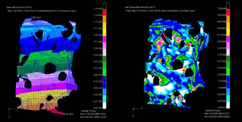
Design FEAts Besides enhancing visualisation, the ultimate aim in 3D modelling is to create digital representations of the putative finished product - and to use these to simulate the proposed function of the object (Working Model 4D) or to perform Finite Element Analysis, eliminating design flaws at the earliest possible stage. To do so, the digital geometry and topology of the object has to be correct - ie, boundaries must be viable, tangents must meet surfaces, surfaces must comply with recognised standards (STEP), and lines and thicknesses must be complete and accurate. Actually, accuracy is more important within finite element analysis than motion simulation - the latter is merely an extension of the cartoonist's craft, where a number of successive pages with slightly differing drawings are printed to the screen. Inconsistencies will occur when data is imported into one system from another, especially where that other system - possibly based on another kernel - is using different standards of accuracy,. Bad communications can also create anomalies in the data. Peter Kerwin, Parasolid's business development manager, calculates that up to 20 per cent of models imported into applications using its kernel software contain errors that have to be accommodated for before they can be used. Parasolid works to an accuracy of 10-8, in a world size of 103, giving an accuracy range of 1011, which is an order of magnitude above other kernel modellers (ACIS, for instance, can create models with a magnitude of 104, but has an accuracy of 10-6, resulting in an accuracy range of 1010). Unit sizes, are, of course, entirely arbitrary in each case, although Parasolid usually works to 1 metre and ACIS to 1mm. CAD developers using either of the kernels set their own units, of course, but I believe, like Parasolid, that 1 kilometer sized models (103 units) represent a reasonable maximum size of model for most purposes. Within the Parasolid kernel, there exists a series of functions that tolerate a certain amount of inaccuracy in imported data. This feature has been called Tolerant Modelling. It enables Parasolid to accept models with an accuracy of no greater than 10-4, closing gaps in boundaries, sorting out multiple intersections and eliminating spikes. More advanced eradication of anomalies, however, needs to be dealt with by a more powerful tool and Parasolid, therefore, has released a set of utilities, called PS/Bodyshop, that incorporates Tolerant Modelling capabilities, but also adds a number of other functions. PS/Bodyshop - the name is evocative of the makeover and titillation end of the motor Industry - kicks in from within Parasolid-based applications to manipulate data in a number of different ways. Closing adjacent faces and the edges on which they should lie is handled by Geometry Healing, the junctions between each being reconstructed. Tangential edges are healed using 3D Solver through Constraint Based Healing and Geometry Repair sorts out self-intersections and discontinuities in translated geometry. Short edges, sliver faces and duplicate geometry - all features that regularly crop up in imported data, especially older data where numerous additions and deletions have been made in drawings - can be removed and Trimming data, healed to create valid faces, can be successfully converted to solids. Should the user then wish to export the model outside Parasolid's world, then geometrical and topographical features that may prevent subsequent use are kindly removed. PS/Bodyshop is normally installed at the server end of the design group system and, as such, is generally transparent as a toolkit to the user. In operation, it highlights errors of concern, asking the user whether the data shown should be redefined or reconfigured.

PS/STEP, PS/IGES and PS/VDA-Fs Concurrent with its release of PS Bodyshop, Parasolid has brought out its own utilities that provide its users with access to industry standard representations of geometric and topographical data. IGES is an international neutral file format for CAD data. PS/IGES enables bi-directional translation of geometric data in IGES format in and out of other CAD systems. Parasolid has produced an API that enables PS/IGES to be incorporated within any Parasolid-based application. JAMA-IS, an IGES protocol developed by the Japanese motor industry, is supported by PS/IGES.

Translation classes Similarly, STEP is the ISO standard neutral file format for defining model surfaces and enabling the exchange of product model data. Using the AP203 protocol to describe the geometry and topology of CAD models, it has been so defined to allow the interchangeability of data between applications with different storage formats. PS/STEP translates data bi-directionally between Parasolid and STEP-AP203. It can also read STEP-AP203 files and create a model from them. Besides supporting STEP-AP203, PS/STEP also supports AP214 Class II, class III, class IV, class V and class VI entities. PS/VDA-FS translates files between the VDA Surface Data Format Interface format and Parasolid XT. VDA is a German standard for transferring surface data, developed by the German Automobile Manufacturers Association (VDA - Verband der Automobilindustrie). Parasolid API is used as a means of plugging in this translator toolkit as well. IGES is mainly a surface-based system, taking each space and creating a trimmed surface for it. The sheets are held in space relying on implied connectivity only - hence the need for them to be stitched together to create a solid model, using extensive human intervention. Both PS/IGES and PS/VDA-FS allow the user to stitch loose faces or sheets into solid models PS/IGES has numerous features that provide highly accurate translation and exchange of data. The transfer of data can be controlled by tunable parameters, whilst callback functions monitor conversion progress - allowing the conversion to be aborted at any stage. Reader modules check the syntax of IGES files, oversee conversion of IGES entities and monitor sewing of surfaces - and preserve entity, label, colour and layer attributes during translation. Root and subordinate nodes are identified and subsequently converted to Parasolid entities, which are then scaled to meters to conform to Parasolid scales of accuracy. STEP, on the other hand, stores the topology of the object, stating that edges may be co-incident. The data that creates the solid model is already there in B-Rep form (Boundary representation) and, knowing where the edges are, there is no need to stitch the surfaces together. PS/STEP incorporates Parasolid's body checking and tolerant modelling capabilities during translation.

Dual-kernel system A recent convert to Parasolid kernels is Visionary Design Systems, whose IronCAD, formally an ACIS-only system, has now been twinned with Parasolid to become the first dual-kernel system. IronCAD uses both kernels simultaneously, switching back and forth when needed. The principal benefit is obviously the ability to work on models developed under either kernel, even to the extent of combining data from either kernel into a single model. IronCAD enables users to switch from one kernel to the other when problems are encountered in one - say, complex bends - that can only be handled by the other. The nanosecond switch is usually invisible to the user. Parasolid is fundamentally involved in interoperability, a basic tenet of EDM. Although they supply a large number of application developers in the CAD/CAM/ CAE markets, each of these enhances and develops the kernel to suit its own particular needs and idiosyncrasies. This creates, along the way, the little sprites and elves that will cause mischief when users try to swap data with each other. As a principal supplier, therefore, they need to remain at the forefront of tool development, ensuring usability of data from whatever source, with or without their kernel. Parasolid was developed by Unigraphics Solutions and has become a line of business in its own right, developing, promoting and selling its kernel both to associated companies and their competitors. Unigraphics Solutions has Solid Edge and iMan under its wing as additional lines of business (not forgetting Unigraphics, the package, itself). Parasolid's user base in mid-range CAD and CAM, and in high-end CAD systems, includes a host of familiar names. CIMData says that 80 per cent of companies with PC CAM solutions are Parasolid licensees. How many people use Parasolid? According to CEO John Mazzola, the new millennium saw 440,000 active seats installed, heading rapidly towards the half million mark! Parasolid and ACIS each share about 40 to 45 per cent of the kernel solid modelling market, although Parasolid has more end user applications - Spatial's ACIS has a vast number of AutoCAD seats. Most of the ACIS seats are in the low-end 2D CAD market, whilst Parasolid has a higher share of the 3D market. Spatial is developing its interoperability and web-based capabilities, and has recently acquired InterData Access and Sven Technologies to assist them.

Standard arguments Until recently, one of the greatest curses of this industry was the total inability of suppliers to accept industry-wide standards. Everybody thought they had it right and, well, everybody else would eventually have to follow suit. It was also the only means of protecting investments in a very threatening environment. Now, with the ease of whirling data around the globe, comes the imperative for that data to be understood once received. A great deal of current emphasis in EDM/PDM software is placed on interoperability tools. However, core software is being developed by fewer outfits, as it requires vast amounts of resource to produce the highly advanced and specialist tools that are now demanded. Spatial and Parasolid provide the bones for many application software providers who subsequently tweak the core software to suit their own customers' needs. Underlying data structures and practices remain identical, though, boding well for future transparency of data. People will, in future, be able to work better and cheaper, without the need for time-consuming and costly manipulation of incoming data. CU

3D file parasolid

Parasolid is a geometric modeling kernel originally developed by ShapeData, now owned by "Siemens Automation & Drives" former UGS Corp., that can be licensed by other companies for use in their 3D computer graphics software products.

It is used in many Computer-aided design (CAD), Computer-aided manufacturing (CAM), Computer-aided engineering (CAE), Product visualization, and CAD data exchange packages.

When exported from the parent software package, a Parasolid commonly has the file extension .x_t. Most Parasolid files can communicate and migrate only 3D solids and/or surface data - Parasolid files currently cannot communicate and migrate 2D data such as lines and arcs.

http://www.plm.automation.siemens.com/en_us/products/open/parasolid/index.shtml

format 3D stl

3D-Formats Programs

(*.stp) STEP-Files (optional)


most 3D-CAD Programs


(*.igs) IGS-Files (optional)


most 3D-CAD Programs


(*.vda) VDA-Files (optional)


3D-CAD Programs


(*.sat) SAT-Files (optional)


3D-CAD Programs


(*.x_t; *.x_b) PARASOLID-Files (optional)

3D-CAD Programs

(*.stl) STL-Files


most 3D-CAD Programs

(*.wrl) VRML1, VRML2-Files
most 3D-CAD Programs


(*.slp) Render-Files


Pro Engineer


(*.xgl *.zgl) XGL-Files


SolidEdge, SolidWorks, Autodesk Inventor


(*.obj) OBJ-Files


Alias Wavefront


(*.3ds *prj *.pli) 3DS-Files


3D Studio


(*.asc) ASC-Files


3D Studio


(*.dxf) DXF-Files (3D-Faces)


(*.iv) Inventor-Files


2D-Formats

Programs
(*.dxf) DXF-Files
most 3D-CAD Programs

(*.dwg) DWG-Files AutoCad, most 3D-CAD Programs
(*.plt, *.plo, *.hpg) HPGL-Files HPGL/HPGL2 Data – Files made by printing data to a file - possible on every PC with a HPGL compatible printing driver.

Export


Formats Content

(*.exe) Viewer+Data

Viewer und Data (3D and 2D)

(*.ddd) Data


Data (3D/2D), Custom Views


(*.stl) STL-Files


triangulated Files (3D)


(*.wrl) VRML 2.0 Files


triangulated VRML 2.0 Files (3D)


(*.3ds) 3D-Studio-Dateien


3D-Studio Files containing the geometrical data of the part (3D)


Recommended File Formats


Pro Engineer:
CATIA:
UG:
SolidEdge:
SolidWorks:
IDEAS:
Autodesk Inventor:
VRML, SLP, STEP, IGS
STEP,IGS,VDA, STL
STEP, IGS, VRML, STL
XGL, VRML, STEP, IGS
STEP, IGS
XGL, STEP, IGS, 3DS, STL

STL 2 SAT parasolid, Transformer du STL SAT parasolid

http://www.cadlink.fr/Default.aspx?tabid=165

XCrySDEN

XCrySDen 


May 31, 2005

The version 1.4 is released. XCrySDen has been ported to MAC OSX (thanks to Mike Ford) and Windows. The former needs X11, while the latter the CYGWIN environment.
  • multi-band display of Fermi surfaces in one widget (read more)
  • visualization of vector-fields with arrows (read more)
  • added support for PWscf v2.1 and later (read more)
  • added support for CRYSTAL03
  • more configurable options for the display of force arrows (color, thickness, aspect) (read more)
  • the color of the "Coordinate system" is configurable (read more)
  • automatic labeling of k-points for k-path selection (thanks to Peter Blaha) (read more)
  • Stereo display mode (thanks to Gerardo Ballabio)
  • Anaglyph display mode, i.e. fake stereo, requires red-blue glasses (thanks to Eric Verfaillie)
  • improved EPS printing (also PDF printing) thanks to new gl2ps-1.2.4. The vectorial EPS printing of Lighting-On display mode is finally good enough.
  • comments added to the XSF format; comment-lines start with the "#" ( read more)
  • dummy "X" (atomic number 0) atoms do not have bonds anymore
  • updated Documentation

vida

VIDA:

VIDA is a graphical interface designed to visualize, manage and manipulate large sets of molecular information. It is capable of handling 100,000s of molecules simultaneously. It supports all standard visualization paradigms, including 2D depiction, both hardware and software stereo, surface selection and manipulation, and many other unique facilities.

VIDA is based on OpenEye's OEChem toolkit and as such handles chemistry properly as well as reading and writing a wide range of formats. The primary features include:
  • A simple and intuitive interface
  • Robust and powerful list manager
  • Chemically-oriented, fully functional spreadsheet
  • Automatic browsing facilities (slide show)
  • List operations
  • Substructure searching
  • Integrated Python interpreter
  • Interactive surface selection/sub-setting, real-time contours
  • Concurrent interaction between data in spreadsheet and 2D/3D displays
  • Multi-level undo
  • Easily save and restore a session
  • Single-click visualization of docking, shape overlay, and electrostatic overlay results
  • Supported on Windows, Linux, Mac OSX, and IRIX systems

Like all OpenEye software, VIDA is available free of charge for non-commercial use.

Sting

What is STING Millennium
STING Millennium is a web based suite of programs that starts with visualizing molecular structure and then leads a user through a series of operations resulting in a comprehensive structure analysis:

amino acid sequence and structure positions,with emphasis on bi-directional coupling of sequence and 3D information
pattern search, neighbors identification,
H-bonds, angles and distances between atoms are easy to obtain thanks to the intuitive graphic and menu interface.
In addition, a user can obtain:

sequence to structure relationships,
analysis of a quality of the structure,
nature and volume of atomic contacts of intra and inter chain type,
analysis of amino acid relative conservation at specified position among homologous proteins, and
Accessible Surface Area
relationship of relative conservation to the intra-chain contacts
functional parameters deciphered etc..

ChemAxon's Reactor

ChemAxon's Reactor.
http://www.chemaxon.com/jchem/examples/reactor/jsp/index.jsp

ramaplot

http://boscoh.com/ramaplot/

MacOSX Universal binary

The Ramachandran Plot Explorer is designed to make it easy to examine the conformation of a polypeptide - through the interactive Ramachandran plot (φ-ψ angles) and χ-angle tool. Simply click on a residue, then drag the marker on the Ramachandran plot.

To see how conformational changes might affect the energetics, I've included real-time calculation of H-bonds, weak H-bonds and steric clashes. This makes it easy to see why (i) certain regions of the Ramachandran plot (what is this?) are forbidden, and (ii) certain sidechain chi angles are favoured, (iii) the core is packed so tightly.

You can also edit (cut/paste/insert) protein sequences and mutate residues, with a simple click of the mouse.

I've worked hard to make an intuitive interface with lots of visual cues and feedback, and I've included what, I think, is a necessary set of navigating tools (sequence-bar, z-slab-bar, snake-measure tool). The program uses native widgets (standard file open/save dialogs!) and you can resize the window to your heart's content.

There is a 3-point-clamp function, that (i) explores discrete solutions of a loop with fixed anchors and 3 hinge-residues, and (ii) allows the exploration of the phi/psi angles of residues inside the clamp without disturbing the rest of the protein.

Limited to a single chain.

qute mol

QuteMol is an open source (GPL), interactive, high quality molecular visualization system. QuteMol exploits the current GPU capabilites through OpenGL shaders to offers an array of innovative visual effects. QuteMol visualization techniques are aimed at improving clarity and an easier understanding of the 3D shape and structure of large molecules or complex proteins.
  • Real Time Ambient Occlusion
  • Depth Aware Silhouette Enhancement
  • Ball and Sticks, Space-Fill and Liquorice visualization modes
  • High resolution antialiased snapshots for creating publication quality renderings
  • Automatic generation of animated gifs of rotating molecules for web pages animations
  • Real-time rendering of large molecules and protein (>100k atoms)
  • Standard PDB input
  • Quick installers for Win and Mac OS X (intel) (new!)
  • Support as a plugins of the NanoEngineer-1 the modeling and simulation program for nano-composites (new!)

pymol macOSX

NOTE: A 3-button wheel or mighty mouse is required to use PyMOL on the Macintosh. Be sure to reconfigure your mighty-mouse to use the secondary button (right-click) and button 3 (middle-click). Tiger (OS X 10.4) is required, although some users have reported success with the final release of Panther (10.3.9).

Option 1: MacPyMOL. MacPyMOL is an Aqua-based PyMOL with a more Mac-like user interface. In addition to supporting native OpenGL rendering, its unique features include Copy-and-Paste of images and direct output of QuickTime movies.
  1. Download and uncompress macpymol-0_99rc6.tar.gz. A Universal Binary
  2. Install by copying MacPyMOL into your Applications folder (or any suitable location).
  3. Launch PyMOL by double-clicking on the MacPyMOL icon.

Option 2: PyMOLX11Hybrid. MacPyMOL now includes a hybrid X11 mode. Assuming that X11 is already installed, simply duplicate and rename the application bundle to "PyMOLX11Hybrid" and then launch (requires Tiger).

<!--Option 3: MacPyMOL for Panther. This is a backwards-compatible release for PowerPC machines running the prior release of Mac OS X.

  1. Download and uncompress macpymol-0_99rc1-panther.tar.gz.
  2. Install by copying MacPyMOL into your Applications folder (or any suitable location).
  3. Launch PyMOL by double-clicking on the MacPyMOL icon.
-->Option 3: PyMOL for Mac OS X / X11. This is the Mac equivalent of the standard Linux, IRIX, and Solaris builds of cross-platform PyMOL. It accesses OpenGL and Tcl/Tk entirely through X11 and is thus completely compatible with the standard version. Requires Mac OS X Tiger with X11 installed.
  1. Download the version appropriate for your system:

    pymol-0_99rc6-bin-macosx-ppc-x11.tgz
    pymol-0_99rc6-bin-macosx-x86-x11.tgz
  2. Extract the archive
    tar -zxf pymol-0_99rc6-bin-macosx-ppc-x11.tgz

    to create a "pymol" directory
  3. Run the setup script from within the new directory
    cd pymol
    ./setup.sh

    to create the "./pymol" launch script.
  4. Then test-launch PyMOL as
    ./pymol

  5. Optional: copy or link "./pymol" to an appropriate location in your path.
    ln -s $PWD/pymol $HOME/bin/pymol

  6. Optional: to avoid having to click twice when moving the mouse between windows, issue
    defaults write com.apple.x11 wm_click_through -bool true

    and then restart the X-server.

chemical drawing software and 3D visu software

MolMol has been cited by over 500 scientific journal articles (search for "molmol" at highwire.stanford.edu). It ranks among the most popular free visualization programs, including RasMol (>700) and KineMages (>450).

http://www.ac-orleans-tours.fr/svt/mol3d/molusc/pcindex.htm

http://dragon.klte.hu/~gundat/rajzprogramok/dprog.html

http://howard.nebrwesleyan.edu/classes/cs295/shoemaker/chem/index.php

http://www.geocities.com/Athens/Thebes/5118/viewdraw.htm

http://www.geocities.com/Athens/Thebes/5118/obc/isis.htm

http://kinemage.biochem.duke.edu/website/kinhome.htm

http://www.pirx.com/iMol/

iMol is a free molecular viewer for Mac OS X operating system. iMol can load molecules using several file formats: PDB, XYZ, MOL2, HIN, CAR, ALC, BIO. The molecules can be saved as PDB, XYZ or BIO files (the BIO file stores all rendering settings, i.e. colors, lighting, orientation of molecules). iMol can easily handle both small and large molecules, it can load multiple molecules, move and rotate them independently.

iMol can load multimodel PDB files and display them as an animation (e.g. molecular dynamics trajectory). iMol supports QuickTime movie format for rendering the animations. The movies are efficiently compressed for web applications.

----

http://www.interprobe.co.uk/inter/interprobe.html

Jmol: (English, Spanish, Dutch )
    Cross-indexing terms:   java applet;   applet;   chime-compatible applet.
Jmol is an open source molecular viewer written in Java. It comes in two forms. There is a Jmol applet which, like Chime, displays the molecule within a web browser. Unlike Chime, you don't have to install a plugin -- Jmol arrives automatically with the web page and displays the molecule. Jmol's second form is a stand-alone application (like RasMol).Because Jmol is written in Java, Jmol runs on a wide variety of operating systems (Windows, Mac OSX, linux, among others) and in all popular browsers (Internet Explorer, Netscape 4/6/7, Mozilla, Safari, etc.). Jmol supports the RasMol/Chime scripting language. The Jmol applet provides a migration path for Chime-based web applications. Jmol includes a perl script which will automatically convert many Chime web pages. The source code and java binaries are available from http://jmol.sourceforge.net and are covered under the GNU Publice Licenses.
    Author: Project, Jmol Submitted by: the author. (Entry 50). Submitted on Dec 14, 2003.
JMolEditor:
    Cross-indexing terms:   java applet;   computational chemistry;   molecular builder;   molecular editor;   gaussian;   gamess, mopac, amber;   vasp;   gromacs;   isosurfaces;   molecular orbitals;   electron densities;   electrostatic potential;   java3d;   picture generation;   BMP;   JPEG;   PNG;   PovRay.
JMolEditor supports submission of Gaussian jobs to remote computer using the ssh2 protocol. It can monitor submitted jobs and retrieve output files after job completion.
---
MAGE: MAGE (available for Windows, Mac, Unix, Linux, and now Java) is the freeware which first brought powerful macromolecular visualization to personal computers (in 1992). Over a thousand excellent tutorials on molecular structures are available in the form of kinemages (presentations that run in MAGE). MAGE has a number of unique and powerful capabilities not available in RasMol nor Chime. (Here is a brief comparision of MAGE vs. RasMol.) There is now a capable Java version of Mage which runs on the Web with no plug-ins. The above page (by Martz) comparing Mage and Rasmol is nicely done in general. However, Mage has ribbons, backbone, ball&stick, etc. representations; kinemages are not scripts but are heirarchical, commented, 3D display lists; and making a simple kinemage is extremely easy, and its exploration is just as open-ended as in RasMol - it's only if you want to make a custom-crafted presentation that it gets "technical". Also, an important use of Mage now is to show all-atom contacts made by Probe
Molecular Workbench: Molecular Workbench is free, content-oriented molecular modeling software for use in education. Unlike the static ball-and-stick models, the Molecular Workbench software computes and visualizes the motion of ensembles of atoms in real time, in both 2D and 3D.
MolViewX: MolviewX is a freeware Macintosh application for OSX that can read several types of coordinate files and display ribbon, CPK, stick, ball&stick, and surface figures. The interface is completely interactive (i.e. no comand line input). There are countless options that control the display colors and characteristics. The output includes object-oriented PICT, QuickDraw 3D 3DMF files, and VRML files. In addition, there are several analysis tools such as neighbors, distance lines, hydropathy plots, Edmunson wheel plots, B value plots (and color coded stick models), distance plots. In addition, the user can open 2 different structures and even perform 3D alignments on them. Also, subsets of the structure can be stored as MOL files and be read in later.
----
http://www.openrasmol.org/
----
POLYVIEW
----
PyMOL Molecular Graphics System
------
http://www.parallelgraphics.com/products/cortonamacosx
Cortona VRML Client for Mac OS X Complete Web3D viewer for Mac OS X!Cortona VRML Client for Mac OS X is a fast and highly interactive Web3D viewer that is ideal for viewing both simple 3D models and complex interactive solutions on the Web. This is a plug-in for Internet Explorer, iCab, Mozilla, OmniWeb and Opera browsers. Cortona for Mac OS X offers:

navigation paradigms (such as walking or flying) that enable the user to move the viewer through a virtual world

a mechanism that allows the user to interact with a virtual world through a sensor in the scene

a hardware renderer based on OpenGL